


How to Think Like a Tree?
And not be a weirdo

Please hug me
When I started dating my (now) wife, I had a silly habit of hugging trees that I considered beautiful. I wasn’t a hipster or a Green Peace activist, or anything of that sort (postwar Bosnia in the early 2000s was not a place for that kind of adventurism). I just liked how some trees looked.
Of course, she thought I was a weirdo so I had to muster all my skills to persuade her that I wasn’t one.
But, I think I had good reasons to be fascinated by the shape of trees. I mean, how can you not like them?
Check this Angel Oak in Charleston, South Carolina, for example:
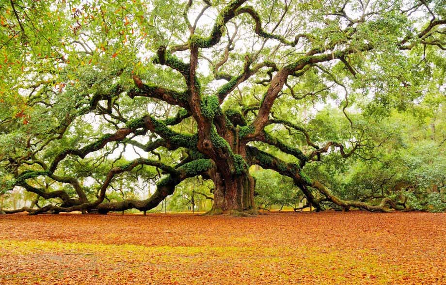
Isn’t it beautiful?
Trees are not just plants; they are also super useful concepts. My fascination with trees quadrupled once I understood how the idea of a tree can be used to improve our thinking.
Now I hug virtual trees, and my wife thinks that’s not as weird.
Tree as a thinking device
This lesson focuses on the concept of a tree as a thinking device. We’ve already talked a bit about decision trees in our modeling lesson, and now it is time to dive deeper.
Let’s start by looking at an example of a decision tree again. This time, let’s try to model a decision-making process about whether to bring an umbrella with us on a random day.
It might look like this:

It is a very simple tree, but enough to start learning more about the basic elements of decision trees.
First, the starting box where the initial question is asked is called a root:

I know, it is weird because tree roots are usually at the bottom, but the decision trees are upside down: the root is at the top, and the leaves are at the bottom.
Next, the middle layer is called a branch:

So, our tree has two branches. Finally, at the bottom layer, we have the leaves:
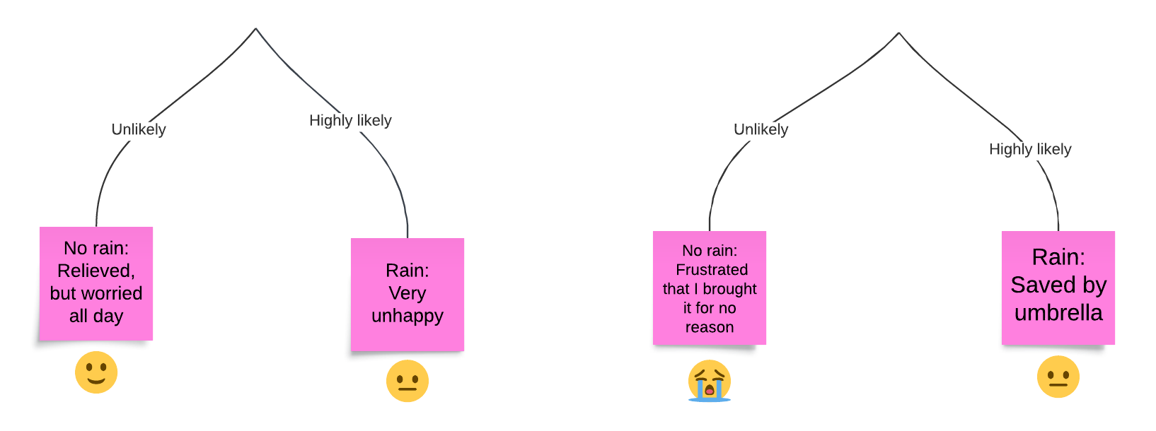
As you can see, there are four leaves in this tree.
Types of decision trees
Decision trees can be used for a variety of situations. Here are some of them:
Modal trees
This simple umbrella example is great for showing how decision trees can aid our decision-making about some simple questions involving multiple scenarios.
The leaves show us the exact number of possible worlds that can occur and tie them to the consequences of our actions at the earlier stages (root of the tree in this case).
It rains in two of these worlds, and the umbrella saves us in just one of them. Similarly, it doesn’t rain in two other possible worlds, and the umbrella is a pain in the ass to carry in one of them.
Classification trees
Trees can be used to classify some objects into larger categories. If you remember the previous lesson, you’ll know that we can use certain features to distinguish between objects and put them in different sets.
Here’s an example of using a decision tree to classify a book:
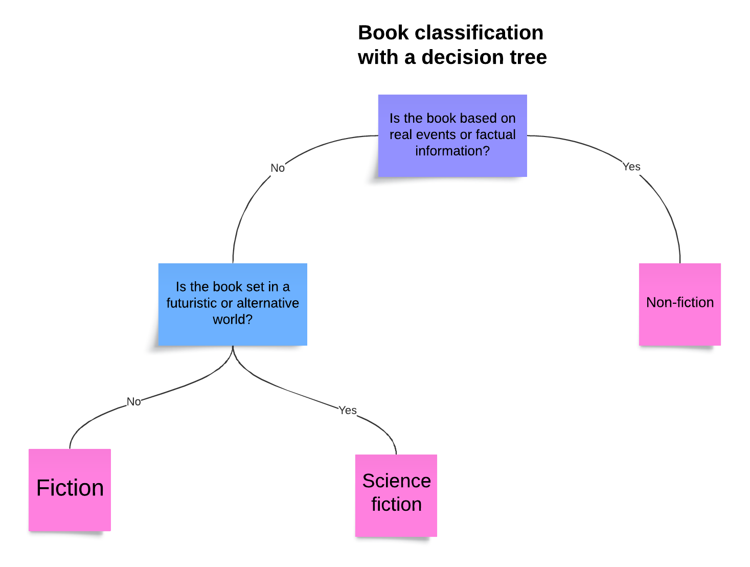
It’s a very small tree, with just three leaves and two main categories (including one sub-category).
Exercise 1: Make a classification tree for anything. It can be a sport, a personality, type of animal, or a hobby. Feel free to use any software. To make mine, I used Lucid, it is free and simple.
Sequential trees
Trees are awesome for representing decision-making processes that require several steps. In life, we rarely make a single decision in any situation. More often than not, each action is built on several small decisions.
Here’s a simple example in the case of deciding what to cook:
As you can see, the number of leaves can grow exponentially, depending on the levels (or the depth) of the tree, and the number of possible options that we’re dealing with. But, even in cases of complex and ‘leafy’ trees, the amount of clarity and organization we acquire by presenting the information in the form of the tree is unparalleled.
Exercise 2: Use the information from the 'cooking tree' and try to present it in some other format, not using the tree. Choose any way to present it; it can be a short text, bullet points, a table ... etc. Compare it to the tree version.Using trees for logical reasoning
Classical critical thinking is built around two main types of reasoning: deductive (logical) and inductive (statistical). Trees can be used to successfully model both of these.
Let’s start by looking at the deductive reasoning. This type of reasoning is very simple. It focuses on the relationships between statements and admits only two truth values: true and false.
For example, let’s take these two statements:
A: EITHER it is raining right now, OR it is sunny.
B: It is NOT raining right now.
If you recall the lesson about truth, you will notice that statement A is a compound statement; it consists of two separate statements (“It is raining right now” and “It is sunny”) connected by logical operators (EITHER and OR). This is known as a disjunctive statement because it works like a watershed: only one of its parts (called disjuncts) can be true.
Statement B looks like a simple statement, but if you look closely you’ll notice that it contains a logical operator (NOT), which is paired with one of the disjuncts from A (“It is raining”).
Let’s presume that both of these statements are true. In that case, we can easily generate another statement, let’s call it C:
C: Therefore, it is sunny right now.
Deductive reasoning is the process of deriving new statements from the information we already have at hand. If you think carefully about the A, B, and C statements, you will realize that statement C was already contained in the combination of A and B. In that sense, deductive reasoning is not ‘inventing’ any new knowledge. Instead, it helps us squeeze all possible information contained in the collection of truths we already possess.
Deductive reasoning, when done correctly, is perfectly ordered; there is no ambiguity in it, it’s entropy (as a measure of disorder) is zero.
Of course, not every collection of statements will have more to be squeezed out of them. These two, for example, are not bearing any further fruit:
D: I love watermelon.
E: IF today is Tuesday, THEN I have to work.
What makes some collection of statements fruitful is how they relate to one another. The A, B, and C statements are structurally connected. This connection can be best seen by using a simple two-leaf tree:
If we know that only one can be true, and we exclude the left leaf, then we can be sure that the right leaf is true.
Trees can help us make sense of other types of connections between statements. In critical thinking, these connections are also known as arguments, and there are several ways to make them. Think of them as different types of structural connections, or ‘argument patterns.’ The one we just saw is called a ‘disjunctive syllogism’ because it involves disjuncts, statements that exclude one another. The most famous of these argument patterns is Modus Ponens, an argument pattern involving conditional statements.
It goes like this:
A: IF it is raining, THEN there are clouds.
B: It is raining.
C: Therefore, there are clouds.
You can recognize that the statement A is the conditional statement because of its use of IF and THEN logical operators. These operators separate the statement into two parts, the antecedent (“it is raining”) and the consequent (“there are clouds”). Statement B then affirms that the antecedent from A is true. Based on these two, we can derive a new statement C that there are clouds.
As a tree, this argument pattern looks like this:
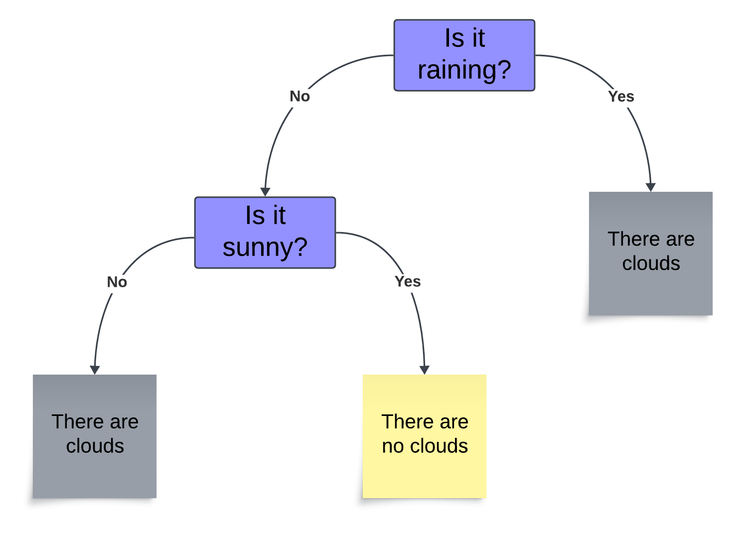
Why can we be sure that the conclusion in statement C is true? As this tree shows us, if the answer to the question “Is it raining?” is yes, then there is only one leaf available, the one affirming that there are clouds.
But, what happens if we change the statement B a bit, and instead of affirming the antecedent from A, we deny the consequent, i.e. we say:
B: There are no clouds.
Can we be certain that it is not raining? Absolutely. As the tree shows us, in case of no clouds, we can be sure that it is not raining. When we go ‘upstream’ from the leaf, we arrive at the information that it is sunny. Since there is only one ‘sunny’ leaf, and since that leaf only leads to the branch containing the information that it is not raining, there is no ambiguity, entropy is zero.
Exercise 3: What happens if in statement B we affirm the consequent from A and say that "there are clouds"? Can we be sure that it is raining? Similarly, what happens if we deny the antecedent from A and say that "it is not raining"? Can we be sure there are no clouds? Explain your answer.
This is a very simple (perhaps too simple) example, but imagine a situation involving more complex and numerous conditions, where the sheer number of results overwhelms our reasoning capacities. In such situations, the tree will help us make good conclusions.
Exercise 4: Make a tree modeling this situation:

A: If it is raining, then the event will be moved indoors.
B: If it is sunny, then the event will be held in the park.
C: If the event is indoors, then free popcord will be provided.
D: If the temperature is above 30°C, then the event will provide free water bottles.
E: If you eat popcorn, then you will drink a lot of water.
Using trees for statistical reasoning
The most amazing power of the trees comes from their use in statistical (inductive) reasoning.
Unlike deductive, inductive reasoning cannot give us certainty in our conclusions; we only have more or less confidence in the truth of our claims, based on probabilities. We cannot achieve full order, and there will always be some ambiguity.
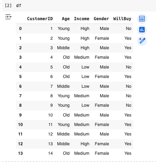
Let’s see an example of this. Imagine you’re a store owner and you tracked how 14 people who frequented your store in an hour behaved, i.e. whether they bought anything or not, so we have some data about customer behavior. Imagine you also noted other information about them, like their age, income, and gender.
See the table below:

This is a data frame, a type of data that contains a lot of information in a neatly organized form. We have four features for each of the 14 customers, and this allows us to gain some insight into how these features relate to the last column: willingness to spend money in your store.
While data frames are amazing as ways to organize information, they don’t give us easy answers. Look at the table above. Can you conclude which type of customer is more likely to spend money?
Not so easy, right?
But, we could use a decision tree.
Check this out:
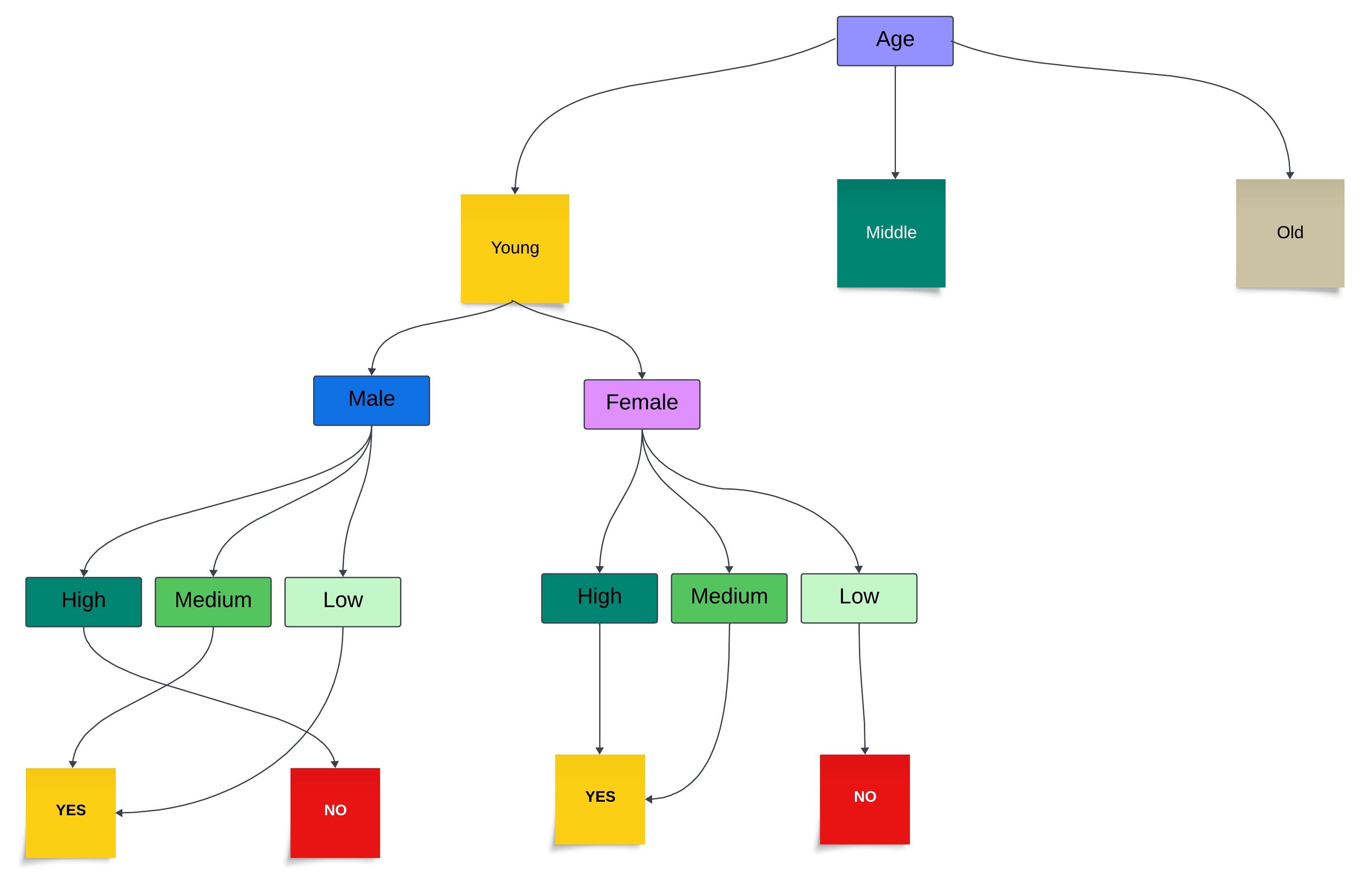
We can use the tree to simplify the information from the data frame and make the patterns more visible to the naked eye, providing us with valuable insight. In this (truncated, due to size limits) tree, we can see that, for example, young females of high and medium income do spend money in the store, while young males of high income do not.
This tree is a simplified and a hypothetical example, and it assumes that there are no instances outside the pattern. Of course, even in the presence of clear patterns, some instances will not align fully with them. For example, we can have one or a few males of high income who make a purchase, or a few women of low income who do the same. In such a case, we will have some disorder in the data.
So, what can we do to decrease this disorder?
The power and beauty of trees is that we can rearrange the way they display information. We can change the decision rules by setting a different feature to be the root of the tree.
For example, instead of age, we can root the tree at “Income”, like this:
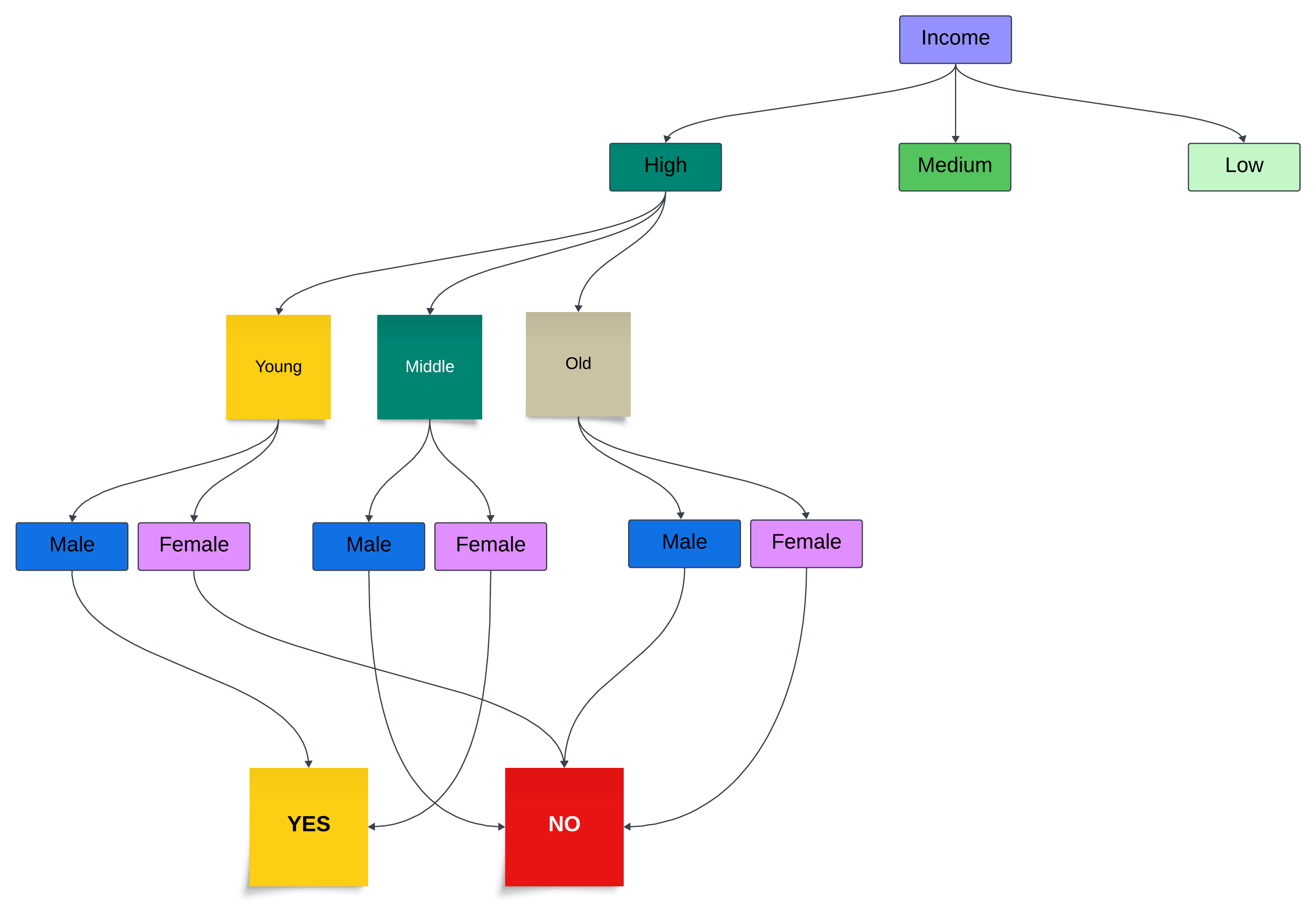
In other words, we can use any possible organization of the tree to gain the most useful insight into the pattern of customer behavior.
We can also drop some of the information if it is not useful. For example, we can organize our tree like this:

Now, the million-dollar question is: which organization gives us the best insight?
The concept of entropy can help us figure that out.
Remember the first lesson, where we introduced the concept of entropy? If you don’t, read it here. To remind you, entropy is a measure of disorder. It helps us calculate how much disorder there is in any system. We can use it to calculate which of the possible organizations of the tree is the most orderly, and thus, contains the maximum amount of information we can get.
How do we do that?
First, let’s define some things in our customer behavior dataset. Since we’re ultimately interested in whether the customers will spend money or not, our target feature is “WillBuy.” That is the class we’re interested in. We’re in business of classification here.
Second, datasets that contain classification information can be pure or impure.
Purity refers to the extent to which a dataset (or a subset of it) contains instances of only one class of the target variable. A dataset is considered pure if all instances belong to the same class, and impure if it doesn't.
For example, in our dataset, the target (“WillBuy”) column contains 9 “Yes” and 5 “No” values, and by this definition, it is impure. It would be pure if all instances belong to either “Yes” or “No” class.
Selecting a subset of the entire dataset could make it pure too. If we only used two colmns, “Age” and “Gender”, (and made a tree with “Age” at the root), then this subset would be pure because all instances of Old Females would belong to the “Yes” class. It would look like the previous image.
Also, impurity can come in degrees. Some subset could be less or more impure, depending on how are the target classes distributed in it. If the maximally pure set is the one in which all instances belong to one class, then the maximally impure is the one that has equal number of instances in all classes.
Entropy is about order, and with order comes predictability. A pure set is predictable, we immediately know that all instances belong to one class; an impure one is not. It is like a flip of a fair coin: we don’t have any reason to think tails or heads are more likely on the next toss.
Entropy is useful here because it gives us a very precise way of determining how pure a dataset is, but also how can we slice it and organize it into a tree to make it purer than it initially is. It gives us an easy way to calculate which ordering of a tree with a certain number of branches (features) has the lowest disorder. By doing so, it helps us reveal the underlying pattern in the data.
It’s time for some math
To see this, we need to understand how is entropy calculated. I’ll show you the formula and explain how simple mathematical concepts give way to an amazing tool for insight.
The formula is this:
First, if you’ve never seen anything like this, don’t worry. I am a philosopher by training, not a mathematician, and it took me a long time to get comfortable with formulas, so I get it if this puts you off.
But, trust me: it is not that complicated, and once you understand it, you will be amazed.
Let’s explain the symbols first. The big weird letter E is a Greek letter sigma and it is used to represent sums. Here it tells us that we sum over many values (from i at the bottom of E to n at the top) of the variable p with a little subscript of i. We will have many ps and we’ll have to sum all of them.
What is p then? In this formula it stands for proportion. In the customer behavior dataset, we have two classes in our target variable “WillBuy”: “Yes” and “No.” This means we only have two ps, the proportion of “Yes”s and the proportion of “No”s. The proportion is just a simple fraction, where the nominator is the number of the members of one class and the denominator is the number of all instances in the dataset.
So, if we have 9 “Yes” in the total of 14 values, the proportion of “Yes” is:
and the proportion of “No” is (remember, we have 5 “No” values):
Notice that the proportion will always be a number between 0 and 1.
Exercise 5: Why is proportion always between 0 and 1? Explain in words.Next, we have the log with a subscript of 2. That is a base 2 logarithm, and it is just a number to which the base (2 in our case) has to be raised to get some other number. If you’re familiar with exponentiation, you’ll have no trouble understand logarithms.
For example, in:
number 3 is the (base 2) logarithm of 8. Or:
In our entropy formula, we sum the products of the each of the two proportions and their base 2 logarithms.
What we’re doing her is basically this:
We multiply the proportion of “Yes” by its logarithm, and the proportion of “No” by its logarithm, and add those two values.
Here is the whole formula again:
We use the little subscript of i to indicate that there could be more ps, not just two as in our current case.
Notice the negative sign before the sum? Since the proportion will always be a number between 0 and 1, its logarithm will be negative. To ensure that our entropy always has positive value (think about why we might want that), we cancel that with another negative sign.
Now, we can proceed with the calculation and use entropy to discover which tree ordering has the least amount of entropy.
First, we have to calculate the entropy of the entire dataset. If S is our entire customer behavior dataset, we sum the two proportions in the target feature (“WillBuy”) times their logarithms like this:
We can use the calculator to compute:
Plugging these values back in:
So, the entropy of the entire dataset is 0.94. This number gives us some measure about how ‘neat’ and orderly is our entire dataset. If all customers fell perfectly into the “Yes” or “No” classes based on their features (like age, income, or gender) then the entropy of S would be zero. If there was absolutely no order, then the entropy in a binary setting like this would be 1.
Our value of 0.94 is close to 1, which tells us that there is a lot of disorder in the dataset, suggesting a large mix of “Yes” and “No” that prevents us from finding some pattern.
Next, since we can split the dataset at each feature (we can use “Age”, “Income” or “Gender” separately and check the proportions of “Yes” and “No” for each) we can calculate the entropy for each of these splits.
For example, the entropy for “Age” is:
Age = Young
Instances: 5 (2 “Yes”, 3 “No”)
Age = Middle
Instances: 4 (3 “Yes”, 1 “No”)
Age = Old
Instances: 5 (4 “Yes”, 1 “No”)
To understand this intuitively, check the ratios of “Yes” and “No” in each of these subsets and compare with the numerical value of their entropy. Notice how the subset that is close to equal number of instances in both classes, like Age = Young, has large entropy, while the subset where most instances are in one class, like Age = Old, has low(er) entropy.
To compute the overall entropy for age, we have to sum these (and weigh them by their proportion in the entire dataset):
What does it mean to ‘weigh’ a value and why we do it? Because in some cases, one subset could be much more (or less) numerous than others, and if it had an extremely high or low entropy it would dominate other subsets. Weighing is achieved here by multiplying the entropy of each smaller subset by the relative size of that subset. It’s something like computing the ‘average’ entropy of the three subsets of the “Age” column.
Next, we do the same with the other two features in this dataset (“Income” and “Gender”). Then, we we compare them to see which one has the lowest entropy. We choose the one with the lowest entropy and set it as the root of the tree. After that, we find the next lowest entropy and set that feature as our next branch, and so forth until we exhaust all our features in the dataset.
And that’s how we arrive at the optimal organization of the tree, which gives us the greatest possible insight into the pattern in our data.
Try it yourself
Computing any of these things by hand is burdensome and takes considerable time. That’s why we’ll use Python to speed up the process.
Now is the time to try this out yourselves.
As usual, open your Google Colab, create a new notebook and define the dataset like this:

If you want to copy-paste the code, use this:
import pandas as pd
import math

data = {
    'CustomerID': [1, 2, 3, 4, 5, 6, 7, 8, 9, 10, 11, 12, 13, 14],
    'Age': ['Young', 'Young', 'Middle', 'Old', 'Old', 'Old', 'Middle', 'Young', 'Young', 'Old', 'Young', 'Middle', 'Middle', 'Old'],
    'Income': ['High', 'High', 'High', 'Medium', 'Low', 'Low', 'Low', 'Medium', 'Low', 'Medium', 'Medium', 'Medium', 'High', 'Medium'],
    'Gender': ['Male', 'Female', 'Male', 'Female', 'Male', 'Female', 'Male', 'Male', 'Female', 'Male', 'Female', 'Male', 'Female', 'Female'],
    'WillBuy': ['No', 'Yes', 'Yes', 'Yes', 'No', 'Yes', 'No', 'No', 'No', 'Yes', 'Yes', 'Yes', 'Yes', 'Yes']
}

df = pd.DataFrame(data)
Let’s explain the code. First, I imported pandas, the Python library required to work with data frames. I also imported the math library, since we will need its logarithm function.
Next, I made a dictionary that will serve as the feed to the pandas data frame function. The keys of the dictionary are variables that will become column names in the data frame, and the values are instances (notice that they appear as lists here, with square brackets) that will appear as rows.
Then, I used pd.DataFrame() with the dictionary as the input to make the data frame, which I creatively named ‘df.’
When I print it out, it looks like this:
Now, let’s make a function that will calculate the entropy of any column in this dataset for us. We can do it like this:
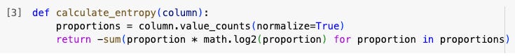
Let me explain the code. If you remember our lesson on functions, you will recall that in Python we first have to define functions before we use (or ‘call’) them. We do so by using the words ‘def’, writing the name of the function (no spaces), specifying what should be it’s input, and hitting the colon. After that, we indent the line and specify what we want the function to do.
Here, the first thing I want this function to do is to find the proportion of each column’s value counts. I call that variable simply ‘proportion.’ Since ‘column’ is the input this function will take, I am setting the proportion variable by appending the method .value_counts() to this input. This calculates the frequency (the number of occurrences) of each unique value in the column.
Check what happens when we use this method on one column. Remember that we can select the column of a data frame by typing the name of the data frame followed by the name of the column in the square brackets, like this:
You can see that it calculated how many “Yes” and “No” value there are in this column.
In calculate_entropy function I also added normalize=True in the parentheses to this method because I didn’t just want the counts; I wanted the counts divided by the total number of values in the column (14 in our case), so I could get the exact proportion. That’s what the term ‘normalize’ means.
Check what happens when we do that:
Now, instead of just counts, we have proportions of each class in the column.
The second line of the function just calculates the column’s entropy by summing all proportions times their logarithm. The slightly odd wording of this line should not scare you. The sum() function is just the equivalent of the weird Greek E letter, and it simply sums whatever is in the parentheses (it should be specified as a list), like this:

Now, our sum() function does not have square brackets but the inside code defines a list because of the way is is worded (this way is called a ‘list comprehension’ in Python, read here more if you want).
Read this line carefully and notice how it says to do something for each proportion in proportions. Here, only the variable proportions has been previously defined, and we are asking Python to go through each value in proportions (for “WillBuy” there are two, as you can see above), which we call proportion (in singular) and calculate the product of each proportion and its logarithm. Then, after all individual multiplying operations are completed, the -sum() function adds them all together (cancels the negative with the minus in front), and return command generates the result.
Let’s see this function in action. When we call it to calculate the entropy of the “WillBuy” column, we get this:

As we found out before, the entropy of this dataset is fairly high. We can reduce it by making a tree that will have lower entropy. To do that, as already specified, we must calculate the entropies of each column (feature) so we can decide where to root the tree. Since we need to weigh the contributions of each subset of the feature by its size, the code will have to be a bit wordy.
Here’s how it will look like:
I’ll explain each line. If you want to copy-paste the entire thing, use this:
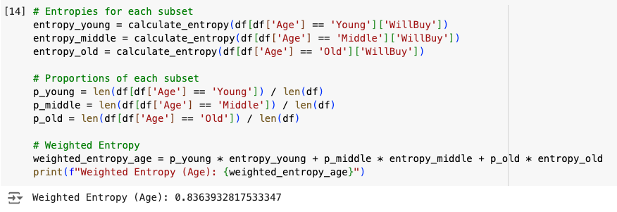
# Entropies for each subset
entropy_young = calculate_entropy(df[df['Age'] == 'Young']['WillBuy'])
entropy_middle = calculate_entropy(df[df['Age'] == 'Middle']['WillBuy'])
entropy_old = calculate_entropy(df[df['Age'] == 'Old']['WillBuy'])

# Proportions of each subset
p_young = len(df[df['Age'] == 'Young']) / len(df)
p_middle = len(df[df['Age'] == 'Middle']) / len(df)
p_old = len(df[df['Age'] == 'Old']) / len(df)

# Weighted Entropy
weighted_entropy_age = p_young * entropy_young + p_middle * entropy_middle + p_old * entropy_old
print(f"Weighted Entropy (Age): {weighted_entropy_age}")
First, I called the calculate_entropy() function for each of the subsets of the “Age” column. Remember that we have three groups here, ‘Young’, ‘Middle’, and ‘Old.’ I select each by using the square bracket selection tool cleverly combined with a Boolean operator that asks whether something is equal to something else (the double equation sign, ==).
You probably notice the weird wording here df[df['Age'] == 'Young']['WillBuy'] where the df part repeats . This is because I first tell Python that I want to select something from the df dataframe. That’s why I open the first square bracket here. Next, I tell Python that what I want selected is the subset of the same df where that subset is the “Age” column (df[‘Age’]) but only for those values that equal ‘Young’ in their value.
We can print only that now, so you can see the result:
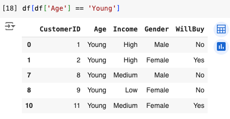
As you can see, this returned the subset of the entire df where the “Age” column contains only the “Young” values.
Next, the code has ['WillBuy'] added after. What this does is it just selects the last column (“WillBuy”) with the “Yes” and “No” values and ignores the rest of this subset data frame.
When we just print that out, here’s what we get:
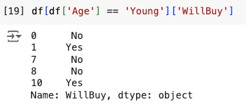
Since this is just one column, and not the entire dataset, it looks a bit different when printed out (it doesn’t come in a one-column table).
Then, we do the same for other two subsets (‘Middle’ and ‘Old’) and set those values to appropriate variables (entropy_middle, and entropy_old).
In the second block, we calculate the proportions of each of these subsets. I used the function len() which calculates the length of anything passed to it as input. You can try this function by itself, put anything as input, even a string, like this:

So, when I wrote p_young = len(df[df['Age'] == 'Young']) / len(df) I created a variable p_young which I set to a number calculated by dividing the length of the subset of the column “Age” whose values are “Young” by the length of the entire data frame.
We’ve seen that there are five young customers in our dataset, so the function len() when called on this subset returns this:
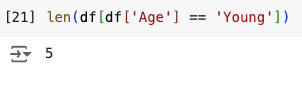
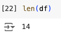
Similarly, there are 14 rows in our entire dataset, so the function applied to the entire data frame returns this:
Finally, the p_young divides the length of the “Young” subset by the length of the entire dataset to get the result of:
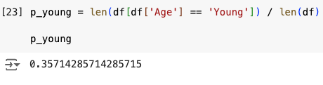
which is just the value we get when we divide 5 by 14.

Finally, the last block of the code calculates the weighted entropy of the entire column according to the way we determined before.
Exercise 6: Calculate the entropy for each of the remaining two columns, "Income" and "Gender." Use the code provided and adjust accordingly. When you do so, compare and see which subset has the lowest entropy. Then, draw a tree with the root at the feature with the lowest entropy, and the subsequent branches with the next lowest entropy value.We’re done for the day
Since there are only 24 hours in a day, we have to stop somewhere, and it turns out it’s right here. This was a very detailed and complex lesson, and there is so much more to be learned about decision trees, Python code, and many other things that would help our understanding.
If any of this was a bit overwhelming, don’t worry. Even if you learned just a tiny bit from this lesson, it is still worth it; you progressed and expanded your thinking abilities. If you have any questions or want a follow-up, feel free to say so below in the comments or in any other, more direct way.
Cheers!