

Hello Darkness, My Old Friend
We all know that many things in life are uncertain.
Will it rain on your wedding day?
Will you ever become rich?
How long will you live?
How often do you think about these things? Does it bother you that you can’t know the answer? Are you afraid of what future may bring?
If you are, you’re not the only one. Everybody faces these fears and frets at the thought of an unknown future.
Although unnerving, the concept of uncertainty is beautiful.
Before studying probability in some detail, I had no idea how nuanced it was. It is hard to grasp, often counterintuitive, and frankly, a bit scary. It forces us to reckon with the reality that no matter how smart we become, there are limits to our knowledge.
The fact is that uncertainty is the force shaping our lives since the day we’re born. There’s no escape.
But what is uncertainty?
In a nutshell, it is the lack of confidence in our knowledge.
I’ll put my professorial cap now and say that, more formally, uncertainty is our attitude toward the truth value of some claims. The lack of definite knowledge about the truth or falsity of some statements creates the condition we call uncertainty.
More poetically, uncertainty is a rupture in our desire to completely order the world we experience; a reminder that entropy is the true master, and we are mere servants.
In this lesson I want to talk about about uncertainty and the ways we can manage it so we can still make meaningful decisions in our life.
Entropy, the measure of disorder, is the key concept here because it helps us understand different levels of order and disorder present in different uncertain situations. If critical thinking is a never-ending resistance to encroaching entropy by creating mental and conceptual order, then the only way to remain a critical thinker under uncertainty is to look for glimpses of order in this chaos.
Randomness
Uncertainty is our psychological and emotional reaction to the underlying fact of reality that some things do not follow a particular order; that they are random. So, in order to understand uncertainty, we need to get a grasp of randomness.
Randomness is a concept that often feels elusive, but it is around us and it impacts our lives in numerous ways. At the core, randomness is the absence of a completely predictable pattern or order.
It is a feature of processes or events. When some process is random, we cannot foresee the its outcome because the process is not governed by any deterministic rules that we can detect.
The most basic example is the one of flipping a fair coin. When you flip it, it can land on either heads or tails, and each outcome is equally likely. This unpredictability is a simple example of randomness; you can’t say with certainty what the result of the next flip will be because there is no predictable order in the behavior of the coin.

Randomness is a concept usually taught in courses on probability and statistics. Besides flipping a coin, many textbooks use playing cards as examples. If you shuffle a deck of cards and pull one of them, you can’t predict with certainty what card will you get.
Randomness is not just about games and experiments. It is a fundamental aspect of many natural processes and phenomena. Consider the proverbial weather: meteorologists can often predict general trends based on some atmospheric data, but they cannot always predict with perfect accuracy what the weather will be at a specific place and at a specific time. The small, seemingly insignificant movements of air, introduce a level of randomness that makes any precise prediction almost impossible.
Similarly, any other phenomenon in life is affected by randomness. How many cars will be on the road today? How many people will vote for candidate X on election day? What will be the price of PlayStation 5 next year?
Randomness is embodied entropy; it is the way disorder manifests itself in the world. But, is disorder a uniform things? Is there only one way for things to be disordered?
Types of Uncertainty
Actually, no.
Here’s an interesting thing: not all uncertainties are created equal. We can be more or less uncertain about the outcome of some event depending on how the underlying randomness is structured.
That is, there is not a single randomness: there are many randomnesses, and some of them are more, and some less structured.
Here’s what I mean by this:
Think of the difference between two games of luck: flipping a fair coin, and tossing a fair die.
If I was to bet you $50, which of the two bets you’d rather take:
You win if the coin lands heads, I win if the coin lands tails, or
You win if the die shows 6, I win if it shows any other number?
If you’re a rational person, you’d choose the first bet.
Why?
Well, because we’re more likely to see a coin landing heads than a die landing 6 in a single flip/toss of both.
Duh!
This right here shows us that despite uncertainty in the absolute truth of some outcome, there are some structural things that help us rein randomness in and reduce the amount of uncertainty as much as humanly possible. Different kinds of situations come with different amounts of entropy, and this provides them with different structures.
What are these ‘structural things’ and how can we use them?
For now, let’s call them parameters. This word usually means something that is kept constant throughout some process or action. Here, it will refer to fixed structural elements of different uncertain situations that determine their ‘amount of uncertainty’, but which can take different values.1
These parameters are important because they tell us a lot about the shape of the underlying randomness.
There are three key parameters here.
Random Variable
‘Variable’ is a term used for anything that varies; in math, variables are non-fixed values, like x, y, and z.
Random variable is a value whose content is random. The outcome of a coin toss is a random variable: it can be either heads or tails.
Random variables have a determined range, and we can describe it by putting all possible values the random variable can take in square brackets, like this:
or
Here, the random variable C is the outcome of a single coin flip, and the random variable D is the outcome of a single toss of a fair die.
Every uncertain situation, by definition, has variables whose content cannot determined, but varies across some range. That’s our first parameter. To understand uncertainty, we first must understand exactly what parameter is uncertain, and what are all the possible values it can take.
Exercise 1: Determine the range of the following random variables:
- The winner of the NBA Championship in a given year
- The year of your death
- The number of of ice-creams you eat in a year
Probability
We can define probability as the long-term behavior of a random variable. Think of it as a fixed feature of a random variable’s character.
Just as some people can be nice or nasty, different random variables can have their characteristic features. For example, the result of a coin flip, a random variable, has the character of landing heads roughly half of the time if we flip it many, many times.
Similarly, the result of a die toss will show 6 roughly 1/6 of the time, if we toss the die many times. These are structural features inseparable from these random variables. That’s our second parameter. Sometimes we know its value beforehand, but sometimes we don’t, and we have to estimate it. But each uncertain situation has an underlying probability structure.
Usually, probability is represented using the letter P in front of parenthesis with the desired outcome within, like this:
or, for the die showing 6:
Exercise 2: What is the probability that the next NBA Champion will be from New York City? Express it as a fraction and use this notation:
P(N) = ...
Explain in one paragraph how did you assign this probability value.
Probability Distribution
If we let random variables ‘play out’ and take the random values within their range for a certain number of times, then what we get as a result is called a probability distribution of that random variable.
For example, if we flip a fair coin 10 thousand times, then this is the probability distribution of the numbers of heads and tails as a random variable:

What this graph shows is that heads occurred roughly 50% of the time in the 10 thousand coin flips.
Observe the Y-axis for a moment. You might be familiar with representing probability on a scale from 0% to 100%, but probability theory actually operates on the range of real numbers between 0 and 1 (inclusive). This is because it is easier to do all the math, and nothing really changes since the quantities remain the same. So, the probability of 0.5 just means 50%, 0.25 means 25% and so on.
To be a valid and reliable measure of uncertainty, probability distribution needs to satisfy three requirements:
Probabilities cannot be non-negative. For example, there cannot be a - 0.5 probability. All probability vales must be equal or larger than 0 and smaller or equal to 1. When the probability of an outcome is 0, then it means that the outcome is impossible; when the probability of an outcome is 1, then it means that the outcome is certain. Anything in between is fundamentally uncertain.
The sum of the probabilities of all possible outcomes in some situation must equal 1. For example, the fair coin flip has only two possible outcomes, heads and tails, and the sum of the two individual probabilities (0.5 each) is 1. Similarly, the sum of all individual probabilities of a die toss (1/6 for each six numbers) is 1.
If the two outcomes in a situation are independent of one another, then the probability that either of them occurs in the sum of their individual probabilities. For example, if you wish to bet that a fair die lands on either 5 or 6, then your probability of winning the bet is 1/6 + 1/6 = 2/6 or 1/3.
So, if we toss a fair die 10 thousand times, then this will be the probability distribution of the results:

We see that, since each number is equally likely to occur, they all have roughly equal probability (1/6 or 0.16666).
It is important to note something you can see on this graph, and that is the fact that no matter how many times we toss the fair die, we will never have an exactly equal number of all numbers, but as the number of tosses increases, they will come very close to being equal.
Now you see visually why betting on the second game is a bad idea - you’d lose 5 out of six tosses on average because my probability of winning the bet would be 5 times 1/6 or 5/6 and yours would be just 1/6.
The concept of a probability distribution is particularly useful because it can help us describe different types of uncertain situations, which in turn can give us a lot of information about the amount and the type of randomness we’re facing.
There are several probability distributions corresponding with different uncertain situations, and we’ll review a few.
Uniform Uncertainty
In situations in which we have several possible outcomes of a random variable and all of those outcomes are equally probable, then we’re dealing with what is called a uniform probability distribution.
Both of the examples we discussed so far (coin flip and die toss) are instances of uniform distribution because each outcome is equally likely. For the coin, both heads and tails have 1/2, and for the die, all numbers have 1/6 probability of appearing.
This is by far the simplest situation, but also the one that has the highest amount of uncertainty and disorder. It is impossible to reduce it further.
Binary Uncertainty
Similarly to the coin, we have other situations in which the outcomes are binary (either X or Y), but in which the probability is not equal, but follows some other distribution.
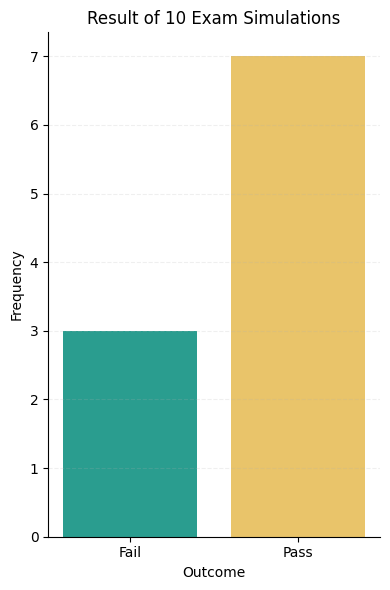
For example, you can either pass or fail the exam (a binary outcome), but the probability of passing it is high (say, 80%) because you’re a good student. This is called a Bernoulli probability distribution, in honor of Jakob Bernoulli, the famous Swiss mathematician.
If you took the same type of an exam 10 times, then you’d pass it 7 and fail 3 times:
Translated to a probability distribution, it would look like this:

In this kind of situation, we have more order, due to the given probability assignment that suggests one outcome as much more likely than the other. If I knew your chances of passing are 80%, I’d happily place a bet that you’d pass the exam.
Repeated Binary Uncertainty
When we have a binary situation with more than one attempt (also called a ‘trial’), then we have what is called a Binomial distribution (which is just a series of repeated Bernoulli-type trials). It is called ‘binomial’ because the distribution is centered around two outcomes, or names (hence bi-nomial), success or failure.
For example, if you’re shooting a hoop 10 times and on each shot your probability of a score is the same (say P(Score) = 0.7, or 70% chance of a score), then this follows a Binomial distribution.
Imagine you repeated your 10-shot experiment 100 times. This would be the distribution of the scores you would make:
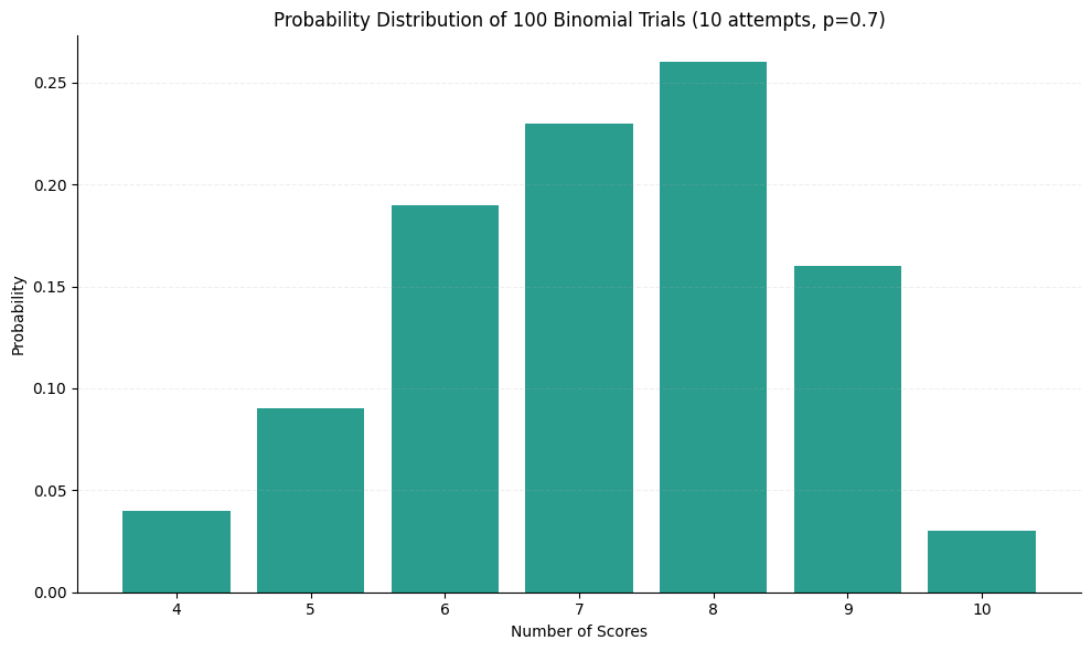
As you can see, you’d probably score 6, 7, 8, or 9 out of 10 shots (with the greatest probability would be of scoring 8 shots, 0.25), but it would not be impossible for you to score just 4, or all 10 of them.
Because the outcome of this little experiment is uncertain, anything is possible. However, the fact that anything is possible doesn’t mean that anything is equally likely. How likely each outcome is depends on the key parameter here: your shooting skill, defined by the probability of scoring the shot. That parameter gives you a footing in ordering your thinking in this kind of an uncertain situation.
Normal Uncertainty
Sometimes the random variables that characterize some uncertain situation do not take whole-number values, like the shot scores or die toss outcomes, but appear on a continuous line, admitting in-between values, like 6.2 or 3.79 or any other real value number. For example, think of the height of all your classmates in school, or coworkers at your job.
In those kinds of situations, other probability distributions are more appropriate.
Now we come to the most important probability distribution you’ll encounter: the normal distribution. It has other names too (‘Gaussian’, ‘Symmetric’, ‘Bell-shaped’) but it is mostly called normal because it occurs in almost every natural situation, from human heights, student test scores, wing-spans in any bird species on the planet, or measurement errors in physics or astronomy. It is very useful in these non-discrete (continuous) situations.
The normal distribution is described by just two simple numbers you learn in a basic statistics lesson: the mean and the standard deviation. For those of you who don’t remember, the mean is also called an average and is calculated by adding all individual values and dividing by the total number of thing measured. For example, if you’re measuring height of 10 people, the average height is the sum of all individual heights of these people divided by 10.
The standard deviation is a measure of how much all the individual values, on average, deviate from the mean. It’s calculation is a bit of a mouthful, so I won’t put it here. If you’re interested, you’ll find it out yourself.
The mean (or average) is known as a ‘measure of central tendency’ and helps us understand what value some random variable gravitates to. For example, if we’re talking about human height, then we know that most humans tend to be around 170 centimeters (or 5 feet 7 inches) tall. We also know that some of them are taller and some are shorter than this. That’s where the standard deviation comes in: it tells us how much, on average, people are shorter and taller than this. Today, the standard deviation of human height is around 10 cm.
Now comes the truly magical feature of normal distribution. Check this out.
Imagine we find 10,000 human beings on the planet and we measure their height. If we do that, then the probability distribution would look something like this:

Because the mean height is 170 cm, the bars are the highest at that point, since most individual measurements ‘gravitate’ towards that value. However, since not everyone is 170 cm tall, many people are either shorter (bars left of the center) or taller (bars right of the center) than this. How many bars will be on the sides of the center depends on our standard deviation, which is 10 cm in this case.
Do you notice anything particular about the shape of this graph?
Maybe if we measure the heights of 100,000 people it would be more obvious? Let’s check it out:

What we notice is a distinct ‘bell’ shape. We can plot a line over the bars so we can see it nicer:
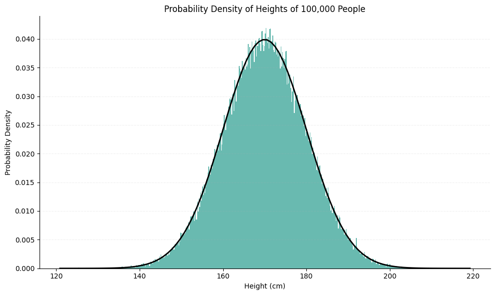
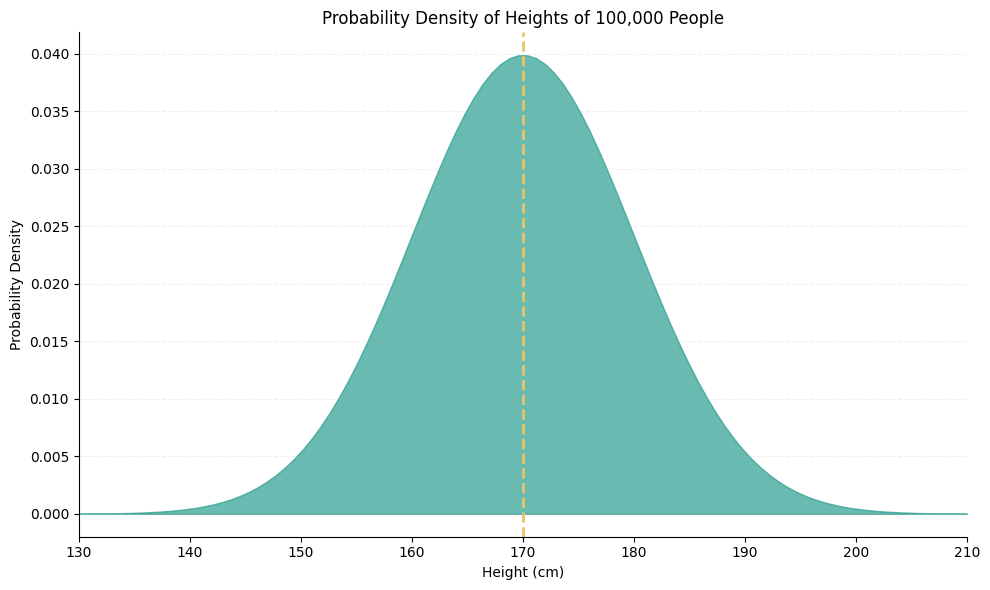
Because human height, like many other natural phenomena, comes in all possible in-between numbers, it is often more appropriate to just represent this with the bell-shaped area under the line, completely ignoring the bars underneath (or pretending that the bars are so tiny so they all merged into a single indistinguishable shape), like this:

I want you to look at this graph carefully. Stare at it until your eyes bleed. Because they will once you understand its magic.
This shape is one of the most important artefacts of our attempts to understand uncertainty and work our way around it.
It is amazing just how much mileage in making decisions under uncertainty we can get with this shape, aided by the two statistical devices we mentioned earlier, the mean and the standard deviation.
Let’s see how.
First, notice how the normal distribution is symmetric around the mean. This means that half of the values of this random variable are below, and half are above the mean, like this:
So, if you meet somebody on Tinder (or LinkedIn, or any other dating app of your choice, I don’t want to be judgmental here) and you’re arranging a date but you’re unsure of their height, you can be sure that there is a 50% chance that they’re shorter than the average human being.
Since you are a smart probabilistic thinker by now, you also know that there is also equal chance that they’re taller than the mean, since the shape is symmetric and the sum of all possibilities in a probability distribution is 1 (0.5 + 0.5).
Here’s another mindblowing fact. We can use the standard deviation to delimit the central area of our distribution by setting the lower and upper limits like this:

This central (shaded) area represents all the values of the random variable within one standard deviation above and below the mean. It covers 68% of all values of the random variable.
Going back to your Tinder date, this tells you that there is 68% chance that your date’s height will be roughly somewhere in this range (160 - 180 cm).
But, wait, there is more.
If now we use two standard deviations, we get this:

In this case, 95% of all the values lie in this range. You can rest assured that your date is in this height range with staggering 95% probability.
Mathematically, one of the most interesting things about this shape is that the area under the bell curve sums to 1. You can use this to calculate your chances that the date is taller than 190 cm, or shorter than 150 cm.
Exercise 3: What is the probability that your date is taller than 190 cm?If you know calculus (or a bit of Python), you can easily find the probabilities that your date is in any possible height range.
Reducing Entropy
So, although uncertainty reigns and you can never know the exact value of some variable in an uncertain situation, you can still make some guesses based on the underlying probability structure of that situation.
Statisticians and data scientists have, over the years, discovered amazing methods to create some order out of the chaos of uncertainty to help us understand reality better and make decision that, while admitting risk that comes with fundamental randomness, aim at achieving the best possible outcomes.
The way to do that is to begin by understanding the nature of the uncertain situation we find ourselves in, determine what variables in it are random, what is the range of values they can take, and what is their probability distribution. Once we establish that, we can choose our actions accordingly. Reducing entropy to zero is impossible, but we can still reduce it to its lowest possible level.
Practice randomness with Python
Before we end, I want you to practice generating some random variables with Python.
We will use numpy, a great Python library for different kinds of numerical manipulations.
So, open up your Google Colab notebook and start by importing the library, like this:

Uniform Distribution
We will start with a uniform distribution. Let’s say we want to generate 10 random real numbers between 0 and 1.
We do it with this code:

Now, when you run this code in your notebook, you’re very likely get completely different numbers because they are, well, random.
In case you wanted 50 random numbers between 1 and 5, then you’ll change the arguments within the np.random.uniform() function, like this:

If instead of real numbers you want to generate integers, you can do it using the function np.random_randint(), Here I generated 10 integers between 1 and 100:

Let’s see what happens if we run this code for uniform integers in the range between 0 and 10 for 10 thousand times. By probability rules we should see each of the numbers in this range selected in a roughly equally number of times.
We will first run the simulation for 10 thousand times and then we’ll plot it using the matplotlib.pyplot library.
Here’s the code:

If you want to copy the code, use this:
import matplotlib.pyplot as plt

uniform_integers = np.random.randint(0, 10, 10000)

counts = np.bincount(uniform_integers, minlength=10) # This counts how many times each integer was selected

plt.figure(figsize=(3, 3)) # This sets the size of the graph to 3 x 3
plt.bar(range(10), counts, color='purple') # This makes the bar graph, setting the range (10 values), using counts and setting color
plt.title('Uniform Distribution of 10,000 Random Integers Between 0 and 10')
plt.xlabel('Integer Value')
plt.ylabel('Frequency')
plt.grid(axis='y', linestyle='--', alpha=0.7) # This sets the grid on the graph
plt.show()
As you can see, each number was selected roughly equal number of times (around 1,000). Although the number selection is truly random, when the simulation is repeated a huge number of times, the distribution reflects the underlying probability structure.
Bernoulli distribution
Now, let’s generate random numbers that follow the Bernoulli distribution. Remember, this one models a binary outcome.
Here’s the code:

Here we set the probability of success at 0.7 (equivalent to 70% chance) and run it as a single instance of a binomial simulation for 10 times (remember that Bernoulli is a special case of Binomial). In this code 1 is coded as success and 0 as failure. So, in 10 Bernoulli trials with 70% probability of success, we had 9 successes and 1 failure.
When you run it in your notebook, you may get a different outcome, but it’s not very likely that you’ll get a radically different outcome.
Here’s the plot:

Binomial distribution
If we have a situation in which we have a binary outcome (success or failure) and the situation involves repeated ‘trials’ (or attempts), for example like in 10 flips of a coin, then we can model it with a binomial simulation.
In the following code, we’re using the same probability of success (70%) and again represent 1 as success and 0 and failure. We run 10 trials of 10 flips each and count how many times we had success (whatever that means in our context, for example getting heads). We then plot it in the similar way:

We see that the most likely outcome is 7 successes, which makes perfect sense since the probability of success is 0.7, but that getting 5, 6, or 8 heads is not unheard of as well. When you run it, you might even get 3, 4, or 9 successes, but not very likely.
Normal distribution
Finally, let us simulate random generation of values of a normal random variable. Let’s imagine that we want to randomly select 10 individuals and we want to check their heights. If we know from earlier that the mean height is 170 cm, with the standard deviation of 10 cm, then our 10 randomly selected individuals will have these heights:

As you can see, I got a few short ones, and a couple tall ones. Your result will, of course, not be exactly the same as mine.
Here’s how it looks like when plotted on the graph (this one is called a histogram and is better for continuous data):

But, if we repeat this ‘trial’ many more times, that is if we select 1,000 instead of just 10 individuals, then our distribution will start getting that characteristic bell shape:

Exercise 4: Think of some other variable that might be normally distributed. For example, find what the mean SAT score in the US among college freshmen and the standard deviation, use the numbers to generate 1,000 scores and plot them using the plt.hist() function as in the graph above.Conclusion
This was a long-ish lesson with a lot of details. This kind of material is usually presented in statistics and probability courses. But, I believe that some basic knowledge of probability distributions is crucial for everyday critical thinking.
When we are faced with uncertainty, it helps to know that each uncertain situation might be unique, at least in the sense of belonging to one or more categories of uncertainty, defined by the underlying structure. Once we get a grasp of this structure, we are able to impose some order to this situation, reduce its entropy and squeeze out as much insight is possible so we can make better decisions.
The bottom line is: probabilistic thinking and decision-making rests on this entropy-reduction process, which starts with finding out the values of the parameters of the uncertain situation - its random variables, probabilities, and distributions - and ends in decisions informed by our imposition of order on the chaos of uncertainty.
I’ll end by a book recommendation. If you’d like to learn more about probability, but you’re looking for a gentle and intuitive book, here’s your best choice at this point:
It’s a very cheap, yet amazing book that will propel your study of uncertainty.
See you next time!
If you’re familiar with this material you might recognize that ‘hyperparameters’ would perhaps be a better term here, but if not, let’s just stick to ‘parameters.’
Thanks for this article. It is quite fluid. The transition from simpler to harder concepts is nicely executed, which enabled me to finish the article and also try the code.