
What is Bayesian Critical Thinking?
Or How to Reason Like a Boss

Thinking is a Process
It doesn’t take a genius to figure out that thinking is not a single event, but a series of them.
First, we never think outside the framework of time; thoughts succeed one another in chunks of time we call moments.
Second, thoughts never exist in isolation; every thought has its genealogy, and we can often track its predecessor.
However, it takes a little bit of effort to understand what the ideal thinking process looks like. We may be aware of the timely and dependent nature of critical thinking, but what is the proper structure of the thinking process? What are its main elements?
In this lesson, I want to examine this process.
Let’s start with the basics.
We Need a Name First
First, let’s decide what we are going to call this perspective on critical thinking.
Since I am not (as my fellow Bosnians would say) ‘inventing hot water’ here, I don’t want to choose a fancy name or take too much credit for the idea.
The type of thinking I will describe here has been around for a while. It is based on an idea Thomas Bayes, an English Presbyterian minister and a statistician had back in the 18th Century when he proposed a novel way to use probability to quantify uncertainty.

Namely, Bayes suggested that thinking, at its core, is about updating our beliefs in a sequential and ordered process: we start with something we already know and then build on it.
Since Bayes introduced this concept two centuries ago, many thinkers followed suit and refined this approach, introducing names for different elements of the idea.
For example, we begin with assumptions, or, as we will call them, prior beliefs, or shorter, priors. These are like default beliefs we have in our minds.
As we go through life, we gather more experience and collect new information (basically, data). We use these data to update our prior beliefs. This new data can either confirm, refine, or challenge those priors.
Once we update our priors with new data, we arrive at posteriors. These new (posterior) beliefs are now our default (prior) beliefs, which we continue updating as we go on.
This is how we generate our understanding of the world, one piece of information at a time. The process never stops, as long as we live. It’s like an intellectual merry-go-round, except that nobody buys you ice cream. You just constantly feel like you were stupid until a moment ago.
This implies a sobering realization: we never fully understand the world. But, that is OK. Nobody expects us to know everything. However, Bayesian thinking helps us keep our beliefs attuned to reality as much as they are humanly possible.
And that is good enough.
That’s the essence of what we will call Bayesian critical thinking: a systematic approach to making better decisions by constantly balancing what we know with what the data say. It’s not just about gathering facts; it’s about evolving our beliefs in light of facts we discover.
In the following sections, we’ll break down this process step by step: the Prior, the Data, and the Posterior.
Where Beliefs Come From: The Prior
Where does knowledge come from?
This is both an ancient and modern philosophical question that can take you, if you’re not careful enough, down a deep rabbit hole.

Tracking down the first thinker who made a claim about the origin of knowledge is difficult, but one philosopher who appears in historical records to have suggested something was Parmenides, a pre-Socratic (read: very, very old, circa 515 BCE) ancient Greek dude. He claimed that knowledge comes from rational thought, not experience, since the world is always changing and our experiences cannot pierce through this constant fluctuation.
This kind of argument was later dubbed rationalism and was picked up by many other thinkers, from Plato to Rene Descartes, and Gottfried Leibniz. They all believed that what we perceive through our senses merely scratches the surface of reality. To get down to the core, we need to use our reason. Therefore, knowledge originates in our ability to think, and not in what we see (or smell, or … taste).

As it always happens in philosophy (and other kinds of pissing contests), there are inevitably some other dudes (surprisingly, it is dudes most often) who disagree.
The alternative view, championed by 18th-century British thinkers such as John Locke and David Hume, is called empiricism. It suggests that human minds are like blank slates (‘tabula rasa’ in Latin) and that everything we know is a result of experience. Adults know more than babies because they have had a longer time on Earth, gathering experiences like Pokemon.

The duty to stick it to all of them and claim that neither group was right fell on a German fella called Immanuel Kant, a weird dude who lived in Koenigsberg (now Kaliningrad) in the late 18th and early 19th Century. He tried to reconcile these opposing views, arguing that while knowledge starts from experience, human minds have some innate structures without which mere experiences would be worthless.
So, knowledge is more like a synthesis of the two: both reason and experience play their part.

I believe that this way of thinking about the origin of knowledge makes the most sense. It confirms what we may realize intuitively too, that we’re never without some knowledge about the world, no matter how inexperienced we are.
Also, no matter how much we know about something, we never know everything and there’s always room for more information.
Cognitive science seems to confirm this view. Our brains are wired to recognize patterns and form priors based on past experiences and try to make predictions about what happens next. These are at the root of heuristics, mental shortcuts our brains make to generate quick judgments.
For example, when you take public transport to work or school daily, you build a mental model (prior) of typical traffic conditions during the day. Based on this model you adjust your timing and choice of transport on each day. If you know that subways are usually the most crowded at 9 AM but busses are less so, then you take the bus.
This belief is your prior. It is like a knowledge default that remains in your mind over a long period.
Priors need not be only deeply rooted beliefs you have since you were born. Anything you believe at any point in time is your prior belief, even if it is based on some experience you had before.
Gathering New Information: The Data
Of course, living in the world means experiencing new things. Every new experience enriches us with additional information about the world. You try a new ice cream flavor, visit another country, meet a new friend, or take a bus at 9 AM. Each one of these experiences brings new data to us.
But, what is data?
The word itself is a Latin plural of ‘datum’, which means fact. So, ‘data’ means facts, or records about the world.
The world is not neatly prepackaged for our consumption, so data don’t exist in some natural state. You can’t pick them up from a tree or catch them in the river. Data are pieces of information about the world that we conceptualize, gather, and organize in ways that lend themselves to analysis.
For example, any piece of data has a type. Let’s say you are a marine biologist and you wish to study the population of Lionfish. What are the types of data that you will use to record how many Lionfish(es) exist?
Numbers, of course.
So, numbers are one type of data. To count distinct objects such as fish, we use whole numbers, AKA integers.
If you’re a climate scientist and you measure temperature, you’d use decimal numbers, such as 90.3, AKA floating point numbers, or floats.
There are many other data types and their usage depends on the nature of the reality we’re trying to capture, some of them as simple as numbers, such as strings (or letters), Booleans (with just two values, True and False), others more complex such as lists, dictionaries, or data frames.
We talked about them in previous lessons.

Data are human-made records that try to decompose and represent reality in the most precise and clear way.
But, data alone are not sufficient to understand the world. We have to make a distinction between data and information. As collections of records about reality, raw data becomes information only when combined with our prior knowledge to shine a light on a portion of reality we’re interested in.
The entire point of collecting data is to update our knowledge: expand on what we believed before we gathered data to advance our understanding of the world. When we combine the prior with the data, we arrive at the posterior.
Updating Our Beliefs: The Posterior
So, how do we update our knowledge using data?
There is no single recipe for this. Much of it depends on the relative strengths of both the prior and our data.
For example, let’s say you are hungry and want to try out a restaurant you’ve never been to before (let’s call it Mike’s Cantina). You don’t have a clue if the food is any good, so you check out reviews on Yelp, and it has 4.5 stars, with most of its 1.2K reviews in the last year saying their fish tacos are amazing.

Based on these reviews you form a prior belief that their tacos are good and you decide to eat dinner there. Let’s say that you take the Yelp rating of 4.5 (on a 1-5 scale) for granted and adopt the belief that the rating precisely reflects the food quality. Think of this as your own, private rating of Mike’s Cantina.
Your prior belief is now that Mike’s Cantina has food with 4.5-star quality.
You sit, order your food, and take a first bite of that fish taco. The taste is not too bad, but it is far from the best taco you’ve had in your life. The tortilla is not the freshest one, the fried fish batter is too salty. You take a few more bites, finish your dinner, pay the check, and leave.
You now have data (the three tacos you ate), and you combine them with the prior to form the posterior belief about the quality of Mike’s Cantina. If you think that the tacos are not as good as the Yelp reviews suggest, you will adjust your own rating of the food in this restaurant. Let’s say that the highest grade you’d give to those fish tacos was 2.0 stars.
Should you then degrade your prior of 4.5 for Mike’s Cantina to 2.0?
Not so fast.
Whether it makes sense to do that depends on the weight of both your prior and the data. The weight here means how strongly do prior and the data pull towards their respective side.
There are three possible ways to model the weight relation between the prior and the data.
First, the prior and the data could have an equal weight. You can imagine a scale like this:
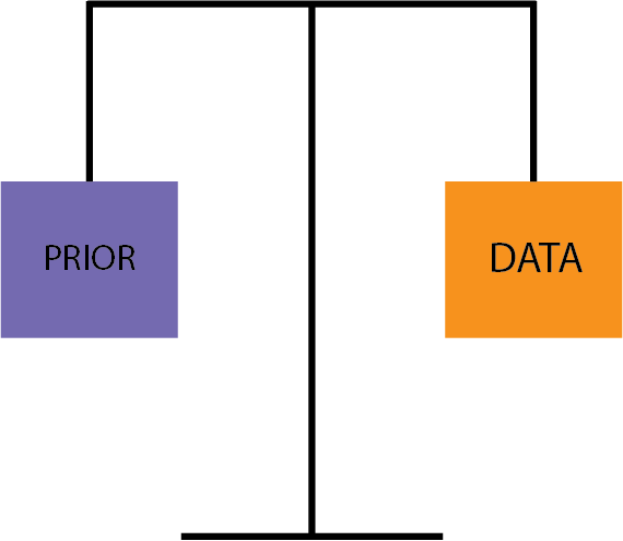
In this case, your posterior is based on equal consideration of both the Yelp reviews and your experience eating those fish tacos.
Second, you might think your prior should be given more weight, so it would look like this:
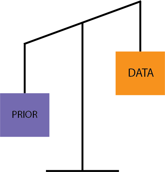
In this case, you’d have more reasons to think that the prior belief is more relevant than your single experience.
For example, you might think that 1.2K reviews reflect the experiences of 1,200 people who ate dinner there throughout the year. Maybe your single dinner at Mike’s Cantina is an aberration - maybe the main chef was sick, or the waiters by mistake brought stale tortilla or some other accidental occurrence happened that doesn’t truly reflect the quality of their food (also, perhaps tacos are not their best dish).
Finally, the third model is the one where the data is weightier than the prior, like this:
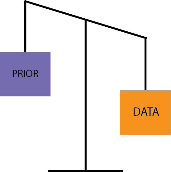
This model would be the best in case you discover, for example, that all those Yelp reviews are false, so your single experience at Mike’ Cantina is more representative than the fake online reviews. Alternatively, you might choose this model in case there were only a handful reviews on Yelp, and you have no reason to assign them too much weight.
As you can see, which prior-data relationship model you will choose depends on the situation, and will significantly affect how much you will degrade your prior rating of 4.5 stars based on the data (your dinner there) that suggested a mere 2.0 stars.
In the first case, since the prior and data have equal weight, you can simply take the average of the prior and the data to come up with your posterior, like this:
So, in this case, your posterior rating for Mike’s Cantina is now 3.25. It is not as high as it was in your prior (4.5), but it is also not as low as your data (your dinner there) suggested (2.0), but somewhere in the middle.
In the second model scenario, where the prior is weightier than the data, you assign the precise weights (you can choose the scale from 0 to 1, for example) to both and calculate the posterior like this:
Here I chose a weight of 0.8 for the prior and 0.2 for the data and I multiplied the respective ratings by these weights. We must choose weights that reflect the relative ratio between the ratings, and we preserve their relation by dividing by the sum of the weights (you can ignore that too since dividing anything by 1 doesn’t change it).
So, if you have reasons to think that your dinner at Mike’s Cantina is an aberration from otherwise a good restaurant, the posterior rating drops only to 4.0 stars after a single dinner.
Collect More Data
Let’s imagine you choose this latter model and decide to give Mike’s Cantina another try. The posterior of 4.0 stars is now your new default (prior) belief about the food quality in this restaurant, and you wish to update it with new data.
You reserve a table, order something else (nachos, for example), and your experience is again subpar. Nachos are not too bad, but you remember having better nachos from a food truck close to your work. You give them a rating of 2.3 stars.
You combine the previous posterior of 4.0 stars (which is now just a new prior) with your new data input (2.3 stars) and calculate another posterior. In this case, since you’ve had two dinners there your data has more weight.
The calculation might look like this:
The prior is still quite weighty (those 1.2K reviews are not meaningless), but not as much as before, since your second dinner counts as more data. The weight for the prior is 0.65 and the weight for the data is 0.35. The posterior now drops to 3.4 stars.
If you’re really adventurous and don’t mind having subpar tacos and nachos, you could choose to continue going to Mike’s Cantina and updating your beliefs about the true quality of food. Each new dinner would be another instance of data that you’d combine with the prior to formulate a new posterior.
The process I just described reflects the nature of Bayesian critical thinking. There are a few important things to understand here:
We always begin with some kind of knowledge about the world, no matter how detailed or strong it is,
Whenever we learn new facts, we balance them together with our previous beliefs to form new, revised beliefs,
How much our new beliefs change depends on the strength of the old beliefs and the strength of the new data,
The more data we have, the lesser weight we give to our prior beliefs,
The updating process never ends,
We never have 100% certainty about anything, new data can change what we think is true.
Exercise 1: Choose a restaurant or a food truck (or any food-selling vendor) you've never been to before and assign a prior rating for the quality, on a 1-5 scale (you can use reviews or if none exist choose some middle-ground prior). Order some food from them and give your rating to that dish. Calculate the posterior based on the weighted average, like we did in this lesson. Repeat the process (if you wish) and update your beliefs.Causal Reasoning
So far, we’ve talked about how Bayesian thinking allows us to update our beliefs based on new data.
But in the real world, our beliefs are often interconnected. What we believe about one thing can influence what we believe about something else: one belief is sometimes conditioned on another belief being true.
In other words, beliefs form networks of causes and effects.
To handle this complexity, we need a way to map these relationships and reason through them logically.
To do that, we can use something called the Bayesian Belief Network (BBN).
This is a neat tool for understanding how different factors or events are causally related. BNNs provide a graphical representation of how various beliefs, causes, and effects are interconnected, making it easier to see how changes in one area affect others. They use the principles of Bayesian critical thinking we described in the first part of this article.
Remember graphs as modeling tools from our previous lesson?

The Wet Grass Example
Let’s make this concept more concrete by diving into a simple, everyday example: the case of wet grass.

Suppose you walk outside one morning and see that the grass is wet. You might ask yourself, “Why is the grass wet?”
There are a few possible explanations:
It could have rained.
The sprinkler might have been on.
Or perhaps both rain and the sprinkler made the grass wet.
To figure out what happened you need to use causal reasoning.
You have two possible causes (rain and the sprinkler) and one effect (wet grass). In Bayesian terms, we would say that our prior beliefs about whether it rained or whether the sprinkler was on will influence how we update our belief about why the grass is wet.
We can describe this visually. In a Bayesian Belief Network, we represent causes and effects as nodes (or circles) and draw arrows (edges) between them to show the direction of influence.
In this case, we only have three variables and their Boolean (binary) values:
Rain (Yes/No)
Sprinkler (Yes/No), and
Wet Grass (Yes/No)
Here’s how we can structure the situation with a graph:
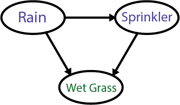
Each arrow in the graph represents a causal influence, meaning that changes in one belief can affect the others.
For example:
Rain → Wet Grass:
If it rained, you’re more likely to find the grass wet. The probability that the grass is wet increases if you know it rained. So, the arrow from ‘Rain’ to ‘Wet Grass’ shows that rain causes the grass to become wet.
Sprinkler → Wet Grass:
Similarly, if the sprinkler was on, it would also increase the chance that the grass was wet. So, the sprinkler is another possible cause for wet grass. If you know the sprinkler was on, this increases the probability that the grass is wet, independent of whether it rained.
Rain → Sprinkler:
This relationship is a bit more subtle but equally important. In some situations, rain might make it less likely that the sprinkler was on. For example, if you have a smart sprinkler system, it won’t turn on when it detects rain. In this case, the arrow shows an inverse relationship—rain reduces the need for the sprinkler.
Now, imagine you observe the grass is wet but don’t know whether it rained or whether the sprinkler was on. The wet grass doesn’t tell you the full story by itself, but it gives you clues. Based on the network, you’d ask questions like:
Did it rain last night?
Was the sprinkler system on?
To reason about causes, we must think backward. Bayesian critical thinking helps us do that by giving us a nice and neat framework for modeling the thinking process.
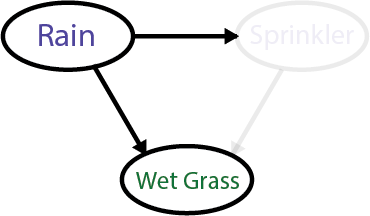
For example, imagine you were sleeping all night and could not hear whether it rained. You open the weather app and see that it rained. Naturally, you conclude that the rain is the most likely cause of the wet grass.
Your reasoning model then looks like this:
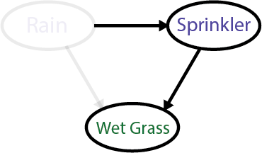
Alternatively, if your weather app tells you it hadn’t rained last night, you’ll conclude that the sprinkler was the cause. Your model would then look like this:
There are two main lessons of causal reasoning that we can learn from this simple example.
First, our beliefs about one thing (the cause of the wet grass in this example) are conditional on other information (data) we have.
For example, given that we know it hadn’t rained last night, we conclude that the most likely cause of the wet grass is the sprinkler. The keyword here is ‘given’ because it indicates that our belief about the cause is conditional on knowing whether it rained last night or not.
Second, any conclusion about causes will be probabilistic, we can never know causes with 100% certainty.
For example, if we know that it had rained last night, we can conclude that the sprinkler was not on and that the rain is the most likely cause. But, can we be 100% sure that the sprinkler was not on? What if it is programmed to turn on every night, regardless of rain?
We can’t know that. That’s why our belief about the cause is probabilistic. We can say that, given no rain last night, we believe with 90% confidence that the sprinkler was the cause of the wet grass.
We use a straight line (so-called ‘bar’ line) to express conditional probabilities in a simple formula, like this:
We read this as ‘the probability that sprinkler caused wet grass given that there was no rain’ is 0.9 or 90%.
COVID-19 vs. Common Cold Example
The wet grass example from the previous section is a staple story from textbooks that teaches you the basics of Bayesian thinking about causes.
Of course, the reality is much more complex than this, but that doesn’t mean we can’t use BNNs to model much more complex situations, with more than three nodes.
Since winter is coming up, bringing us a season of respiratory diseases, let’s try to model a situation in which we try to reason about the most likely cause of some set of symptoms.
Let’s say you wake up one morning with a fever, and you want to figure out if it’s more likely that you have a common cold or COVID-19.
How can we use Bayesian critical thinking to do that?
First, we identify the nodes (variables) in a graph and their binary values:
Common Cold (Yes/No)
COVID-19 (Yes/No)
Cough (Yes/No)
Fever (Yes/No)
COVID Test Result (Positive/Negative)
Second, we identify possible causal relationships:
Common Cold → Cough: A cold can cause a cough.
Common Cold → Fever: A cold can cause a fever.
COVID-19 → Cough: COVID-19 can cause a cough.
COVID-19 → Fever: COVID-19 can cause a fever.
COVID-19 → COVID Test Result: COVID-19 can cause a positive COVID test result.
Then, we identify probabilities:
Prior Probabilities (before symptoms):
There's a 10% chance you have COVID-19 (based on the prevalence of COVID-19 infections in our area).
There's a 30% chance you have a common cold (based on the same criteria).
Conditional Probabilities:
If you have the common cold:
Cough: 60% chance.
Fever: 20% chance.
If you have COVID-19:
Cough: 80% chance.
Fever: 70% chance.
If you don’t have either:
Cough: 5% chance (dry throat, etc.).
Fever: 1% chance (something unrelated).
COVID Test:
If you have COVID-19, there’s a 90% chance the test will be positive.
If you don’t have COVID-19, there’s still a 5% chance of a false positive (meaning you will get a positive test even though you don’t have the disease).
These probabilities will be based on whatever the previous data show. For example, the Center for Disease Control (CDC) usually has up-to-date information about the infection rates for both COVID-19 and the common cold in the US.
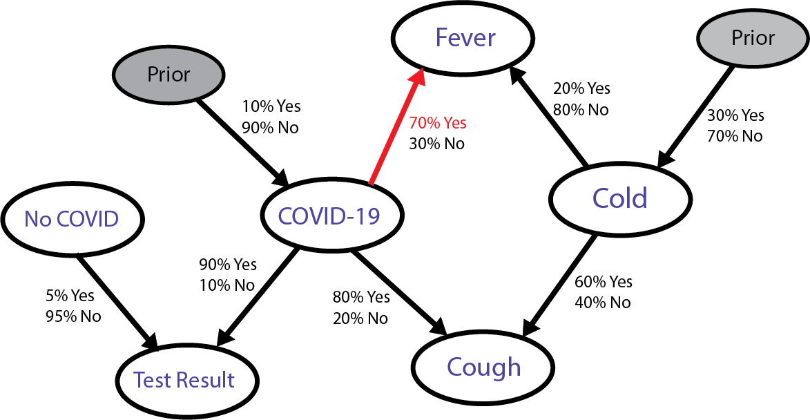
Let’s draw a graph to represent this visually:
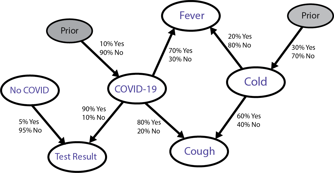
As you can see, this looks much more complex than our wet grass example, which is to be expected, given the complexity of reality about diseases and their relation to the symptoms.
Bear in mind, however, that this graph is still a simplification of reality.
Now, how do we reason about this?
If you have a fever, and you look at this graph, what is the most likely cause of that fever, COVID-19 or common cold?
Since the likelihood of having fever in case of COVID-19 is greater than in the case of a cold, you might rush to say that you are 70% confident that you have COVID.
But, not so fast.
Causal reasoning works backward and the arrows in this graph determining probabilities go only one way (forward), so we have to be more clever than that.
How can we be more clever? Similar to our case of food quality rating in Mike’s Cantina, we’ll have to weigh our numbers and divide them by a sum of weights to figure this out.
Let’s start by expressing some things we know here in symbols.
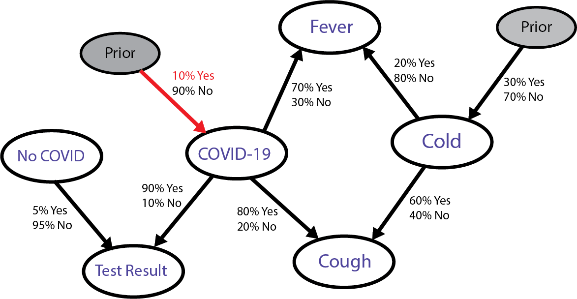
First, the prior probability of having COVID is 10%, or symbolically:
We read this as the probability of catching COVID-19 is 0.10 or 10%.
Similarly, the prior probability of having a cold is 30%, or:
If we look at the graph we see that the probability of having a fever given that we have COVID is 70%.
We write that like this:
Remember that we use the vertical bar to represent conditional information. Note the use of the word ‘given’ to indicate a conditional relationship.
Similarly, the probability of having a fever given that we have a cold is:
Now, since what we are interested in here is the probability of having COVID given that we have a fever, our unknown value can be written like this:
Note that what we wish to know is the inverse of what we already know through data.
How do we figure this out?
Let’s look at the graph again. This time focus only on what nodes influence the ‘Fever’ node, either directly (like COVID and Cold) or indirectly (like the ‘Prior’ nodes for both).
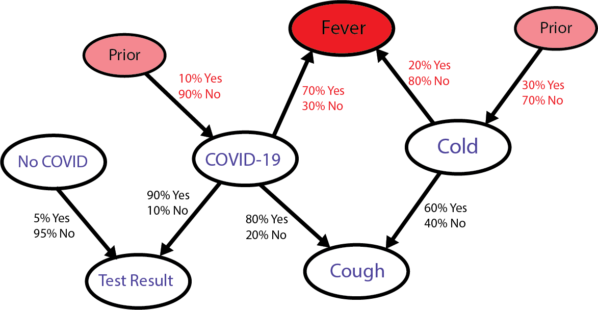
What we need is to determine how ‘weighty’ is the causal relationship between COVID and ‘Fever’ relative to the causal relationship between Cold and ‘Fever’. How do we do that?
To understand what we’re about to do, think about this scenario. If you have two friends, Jake and Mary, and Jake weighs 100 lbs while Mary weighs 75 lbs. How heavier is Jake relative to Mary?
A simple way is just to say that he is 25 lbs heavier.
When we say Jake is 25 lbs heavier than Mary, we know the raw difference, but it doesn’t tell us how significant that difference is. If Jake and Mary were both heavier overall, the 25 lbs might not seem as large (imagine Jake was 1025 lbs and Mary was 1000 lbs).
Instead, we can get a better measure by dividing Jake’s weight by their combined weight, like this:
By dividing Jake’s weight by their combined weight, we get a relative measure. This tells us that Jake is about 0.57 times heavier, meaning he makes up 57% of their total weight. This gives us a better sense of scale—showing how much bigger Jake is relative to the whole.
In short, the relative measure puts the difference in context, making it easier to see how significant it is.
We are going to do the same with our causal example, by measuring the weight of the causal relationship between COVID and ‘Fever’.
We are going to use this formula:
Read this out loud using the guidelines provided above.
Our conditional probability that you have COVID given that you have a fever is a ratio between the probability that you have a fever given that you have COVID, which is this part of the graph,
multiplied by the prior probability of having COVID, which is this part:
That’s what we’re interested in. Whenever we have ‘chained’ probabilistic nodes like this, we use the multiplication of all probabilities along the chained path to calculate their joint occurrence.
However, in order to figure out how ‘weighty’ this causal relationship is, we have to divide it by the probability of having a fever in either scenario. Since we don’t have a prior probability of having a fever, we must add all possible paths to ‘Fever’ from both COVID and Cold side.
We do that by first multiplying each conditional probability from COVID and Cold to ‘Fever’ individually and simply add them together (we already did that in the numerator for COVID, we just add that to the same calculation for Cold). This is equivalent to adding up Jake and Mary’s weight so we determine Jake’s relative weight.
Here’s what that looks like in a formula when the denominator P(Fever) is expanded:
And here’s the graphical explanation:
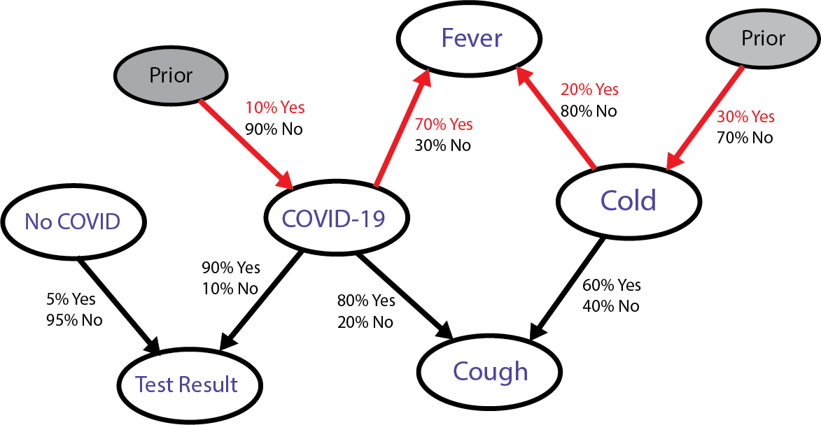
Since we have all the values here, we simply plug them into the formula:
Finally, we get a result of about 0.53 or 53% chance of you having COVID given that you woke up with a fever. So, it is not 70% chance as you might have initially thought.
Exercise 2: Perform the same calculation to figure out the probability that you have COVID given that you have a cough instead of fever. Is it higher?Conclusion
This was a long lesson, and I’m sure you’re exhausted after reading and thinking through all of this.
If this sounds a bit too complex and confusing at times, don’t worry. Bayesian thinking can be dizzying to anybody who learns about it for the first time.
But, as is the case with many things of high level (like climbing Kilimanjaro or Mount Everest), once you get accustomed to the heights, you will see the how awesome is the view.
Bayesian critical thinking is at the root of scientific reasoning. Learning more about it will supercharge your thinking skills.
Exercise 3: You're trying to figure out whether your subway train will be delayed. There are two main factors that can affect whether there’s a delay:
- Rush Hour (Yes/No)
- Bad Weather (Yes/No)
Your task is to use a Bayesian Network to model how these two factors influence the probability of a delay.
Here are your causal relationships:
- Rush Hour → Delay: If it’s rush hour, the chances of a delay increase.
- Bad Weather → Delay: If the weather is bad, the chances of a delay also increase.
Here are your probabilities:
Prior Probabilities:
- Rush Hour: 30% chance.
- Bad Weather: 20% chance.
Conditional Probabilities for Delays:
- If it’s rush hour, the chance of a delay is 50%.
- If there’s bad weather, the chance of a delay is 60%.
- If neither rush hour nor bad weather, the chance of a delay is 5%.
Draw the graph manually and compute the probability that the train will be delayed given that it is raining right now.
For extra credit, write a Python function that takes as input the prior and conditional probabilities, and computes the posterior.
If you want to learn more about Bayesian reasoning in general, here are some useful books to start with:
Amazing and critical read. Critical in this times were machines "Thinking" is evolving exponentially.
Like you said, we build patterns over time based on our experiences and data. Machines do that too, but we do it on a dimension that's not understandable for a machine. The emotional dimension, a computer will never like a tacos restaurant over another, but they can integrate millions of tacos reviews in their system (we cant do that).
Machines capabilities are horizontal, human capabilities are vertical.
I belive it's important to understand this, as we integrate technology into our life and work.
Exceptional explanations with great humor. Graphics helpful and appreciate the book recommendations. Will now be looking for Bayes projects everywhere!