


How to Milk Information?
A Love Letter to Data Frames

When Data is Your Cow
Critical thinking is a modular activity. Every new thought is made out of many other thoughts in our minds. Decomposition, abstraction, pattern recognition, and algorithmic thinking drive our critical reasoning, and they depend on meaningful and careful breaking of ideas into their basic elements.
One of the best ways to see this in action is to learn more about one specific data type: data frames. These are special ways of organizing complex information (about something) into a form that allows us to extract as much insight as humanly possible. To put it bluntly, data frames allow us to ‘milk’ knowledge from a simple collection of facts.

How is that possible? Let’s start by understanding the basics.
What Are Data Frames?
You are probably familiar with data frames, although you may have called them differently. Sometimes they are called ‘data tables’ (or just ‘tables’), ‘datasets’, ‘matrices’, or ‘spreadsheets’, depending on your professional background, age, or the choice of software.
They all look similar. Something like this:

They organize different types of information (such as numbers and words) into a matrix of rows and columns, where each row represents an instance of something (in the above example an instance of a human being, or a person), and each column represents a feature of that instance.
For example, in the example above the column Name is a collection of names of each person, the column Salary is a collection of their salaries. Each row tells us something about one person. So, we learn that Bob is 27, lives in San Francisco and makes $60,000 a year.
It looks very simple, right?
From today's perspective, this looks unremarkable. But, organizing information in this way hasn’t always been around. There is a historical record of some ancient civilizations (such as the Inca) using colored knots on a rope to encode information, using a system called ‘quipu’, as the one below:

However, what we know as modern data frames (at least in some rough shape) hadn’t occurred until the 17th Century, when the pioneer of British demography, John Graunt collected and tabulated information about births, deaths, and causes of death in London parishes, which were published every Thursday by the authorities.

In his ‘Table of Casualties’, diseases are instances in rows, while years are the columns.
Check it out:

Using the tabular format allowed Graunt to estimate the population size of London and England, as well as birth and death rates, prevalences of disease, and similar.
In the 1970s, an Oxford-educated mathematician working at IBM, Edgar F. ‘Ted’ Codd came up with the concept of a ‘relational database’, an organized way of representing information in rows and columns, where each row represents a single record (an instance), and a column the property (or a feature) of that record. Codd’s original idea helped shape modern data frames, introducing relations between rows, columns, and datasets that allow clearer insights into the data.

The guy was so awesome that he came up with an entire algebra for creating and manipulating different data frames, called ‘relational algebra’.
See more here.
His idea gave birth to the modern concept of a database - a collection of mutually relatable data frames - that drives much of today’s technology.
I will not exaggerate if I say that the data frame is one of the most amazing and underrated inventions in human culture. So many of the good things we have today wouldn't exist without them: from medical research, e-commerce, and social media, to cybersecurity.
There would be no ATMs or credit cards without data frames. Nowadays, entire industries and economies depend on them.
Windows to the Mind
Fundamentally, data frames are collections of information, which implies that somebody performed the act of ‘collection’. That is, behind every data frame there is a (living or dead) person who is responsible for the decision about what kinds of information to collect and combine into it.
In that sense, data frames are like windows in the mind of the ‘collector’. Rows show us their central target population (people or inanimate objects), the main point of interest, and columns show us what particular things about this population the collector wanted to know.
So, data frames are subjective perspectives on the world. They are like slices of somebody else’s gaze on our shared reality.
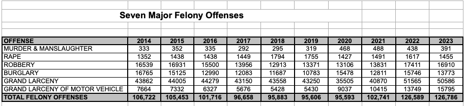
For example, a crime data frame might have information about the types of crime as rows, and years as columns, such as in this data frame about crime in NYC:
Or it might include the racial identity of perpetrators as columns instead, such as in this data frame:
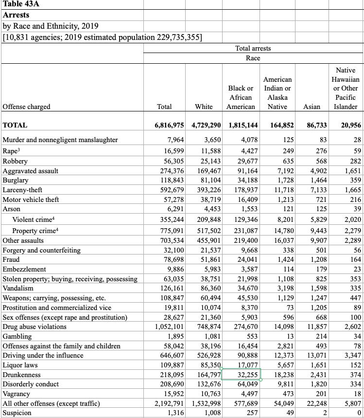
The choice and presentation in data frames is always selective, and it has the power to shape what we perceive as important.
They are never ‘just data’: each data frame tells a story if we’re willing to look carefully. They are narrative by design.
However, this doesn’t mean that they are not true, or that they have equal informational value as a folk tale or something similar. Having exact data about a topic is as close as we can get to truth. However, some collections of data might be too partial (read: insufficient) to provide us with the full picture of that aspect of reality.
Exercise 1: Study the two crime data frames above and write a 3-sentence story based on each. What insights did you gain while studying both?Working with Data Frames
Every sufficiently detailed data frame (one containing more than just one column of relevant and interesting facts) provides us with a great opportunity to extract a treasure trove of information from it.
This practice, which lies at the border of art and science, is called data analysis (sometimes also data mining). How can we extract information from a data frame?
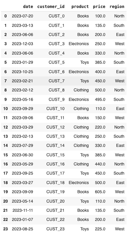
Imagine you are an owner of a big online retail company (similar to Amazon) and you sell a bunch of different products each day. Your sales team keeps a record of each sale and keeps all that information in a data frame that looks something like this (but containing perhaps thousands of rows covering a period of several years):
What do you see here?
Even a quick glance can tell you something.
First, you see that the period in this snapshot of the data frame covers several months in the year 2023. Second, you see that the products sold were mostly clothing, electronics, and toys. You can also see the price and the region where the items were sold.
But, data frames allow us to filter and aggregate some specific information from here in a way that can give us more insight.
We just have to dig deeper.
For example, we can group the average price by region to see which part of the country accounts for most of our revenue and make an additional data frame showing that, like this:
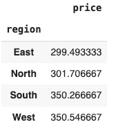
We see here that South and West tend to spend a bit more than North and East.
Or, we may want to see if we have some faithful customers, and where they come from by looking at the best spenders, like this:
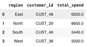
We can see here that there are four customers who spent more than $5,000 in our store. These are our golden geese.
Also, we may want to see which products sell the best, so we group the amounts spent on each product, like this:

We see here that our customers love buying books a bit more than toys.
I hope you can see the power of data frames in this simple example. By combining a lot of individual pieces of information in an organized two-dimensional way with rows and columns, they allow us to represent a much more complex multidimensional reality and derive much more insight from that reality than it is initially available to us.
Just imagine how much can owners optimize their business and increase their revenue by finding out who spends more on their website, in which part of the country, and what products are most popular. That possibility exists only because we have data frames.
Exercise 2: Study the hypothetical retail data frame a bit more. Look at it. What is another piece of insight that you'd want to derive from this data frame, if you were the owner of this business?How to Make a Data Frame?
The best way to understand data frames is by learning how to create them.
There are many software choices at disposal to anybody who wishes to make a data frame. Many people have encountered at least some of them in their lifetime, such as Excel.

But, here we will use Python because it is:
Easy and intuitive to use,
What many data science experts use,
The building block of development of AI.
So, let’s head to our Google Colab notebook and type this:
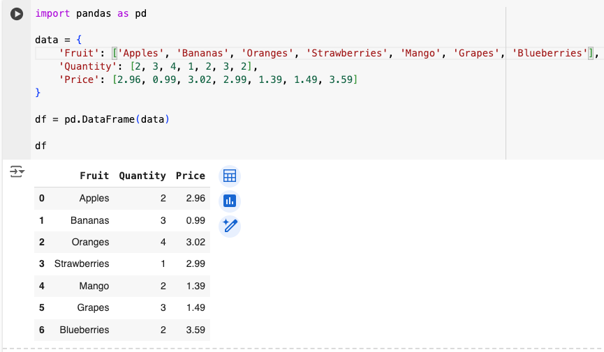
The first line of code that says import pandas as pd is crucial here.
As a programming language, Python is build from the basic Python that was developed by its creators, as well as a gazillion of additions called libraries. These are buckets of code that expand on the basic Python abilities and allow us to do different things with them. Pandas is one such library.
With this line of code we import that library into our notebook so we can use it (we use pd as a shortcut so we don’t have type the entire word Pandas every time we want to use it).
In the second line, we create a dictionary (something you have already learned to do in previous lessons), where each key is what we wish to be the name of the column (‘Fruit’, ‘Quantity’, and ‘Price’) and each value for that key is a list of items of equal length.
For ‘Fruit’ we have a list of fruits, for ‘Quantity’ a list of quantities for each fruit, and for ‘Price’ we have the price of each fruit (per pound, let’s say). Imagine this is your grocery shopping list for a week.
Once the dictionary is made, we create a variable df which will hold our data frame and use the pd shortcut to make a data frame with the pandas library with this code:
df = pd.DataFrame(data).
The pd.DataFrame() is a function that will take a dictionary (here that is data) as input within the parentheses and make a data frame.
Then, we simply type in the name of our dafa frame (df) and we get our data frame displayed below the cell.
And there you go, you just made your first data frame. Congrats!
As you can see, data frames are very useful for combining different types of data in a single packet of information. To see what are these different types, we can peek into the structure of our data frame by using the command df.info() which will display some of the structural information, like this:
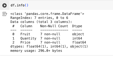
Here we can see that our data frame has 7 entries (indexed from 0 to 6 - Python starts counting from 0), has three columns, where the first column is an object, the second one is an integer, and the third one is a float data type. Objects are usually data types containing words and letters, integers are whole, and floats are decimal numbers.
Exercise 3: Get a receipt from your recent grocery shopping and make a data frame using Python. List items you bought, quantities bought, and price per item. Think of the best way to organize your data frame. What features do you want to have in columns? What instances do you want in rows?The design of data frames is both an art and science. Since data frames are human creations, we get to decide how to make them. What features will be included in the columns, what particular instances will be in the rows - these are not trivial questions and they cut deep into the practice of data design. Since our aim is to use data frames to represent some complex aspects of reality, we need to be smart about how to do that.
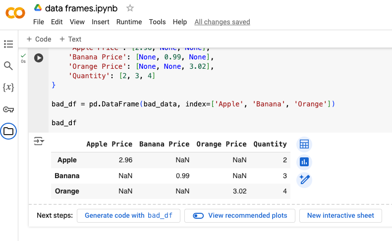
For example, a bad way to organize the same information would look like this:
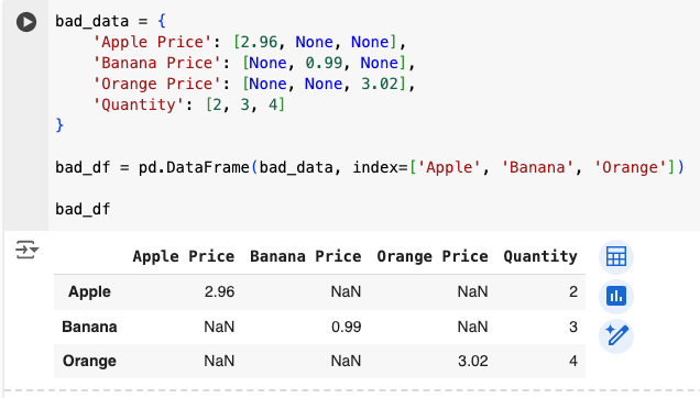
You can tell even by a quick glance that this data frame is not particularly useful. Many values return NaN (which stands for Not a Number), the organization is very bad, and we can get very little insight from it.
Therefore, data design matters.
Importing Data Frames
Making data frames is fun and you may want to do that sometimes. But, more often than not, you will be using data frames somebody else made to derive some insight from them.
Let’s learn how can we import data frames into our Google Colab notebook and perform some basic analysis.
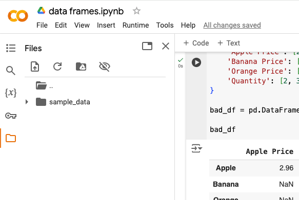
If you look at the left side of your notebook, you’ll notice a little folder icon at the bottom (here circled out in blue):
Click on that icon and a menu of options will appear, like this:
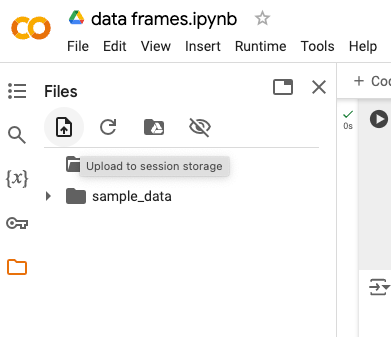
Next, check that icon that looks like a paper sheet with a folded corner with an arrow in the middle.
That’s our link to upload a file.
When you click on it, you will get an option to upload a file to your notebook (to your session storage).
Now, let’s go and find a nice and interesting data frame to upload.
Since critical thinking is a way to resist entropy and since death is an important entropy-point for humans, let’s work with this dataset: leading causes of death in NYC.
Go to the link an download the CSV file (stands for Comma Separated Values).
If you want, click down here to download the file:

When you download this link, go to the Google Colab upload link, click it and navigate to the CSV file you just downloaded.
Once you do that, your file will appear in the notebook, like this:

(Note that I renamed my file to nyc_death.csv before I uploaded it, because the original name was too long and I was lazy to type it).
Now the file is in your notebook memory, and you can access it through the code cell. This file will remain in your notebook memory as long as your notebook is open. If you close it, you’ll have to upload it again.
Now, let’s access it with Python.
We do it like this.
First, right-click on the data frame you just uploaded and copy the path to it:
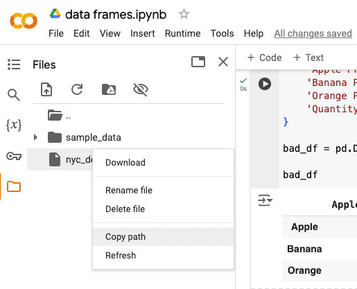
You will need this in the cell in a second.
Then open a new cell and import the file like this (see details below the picture):
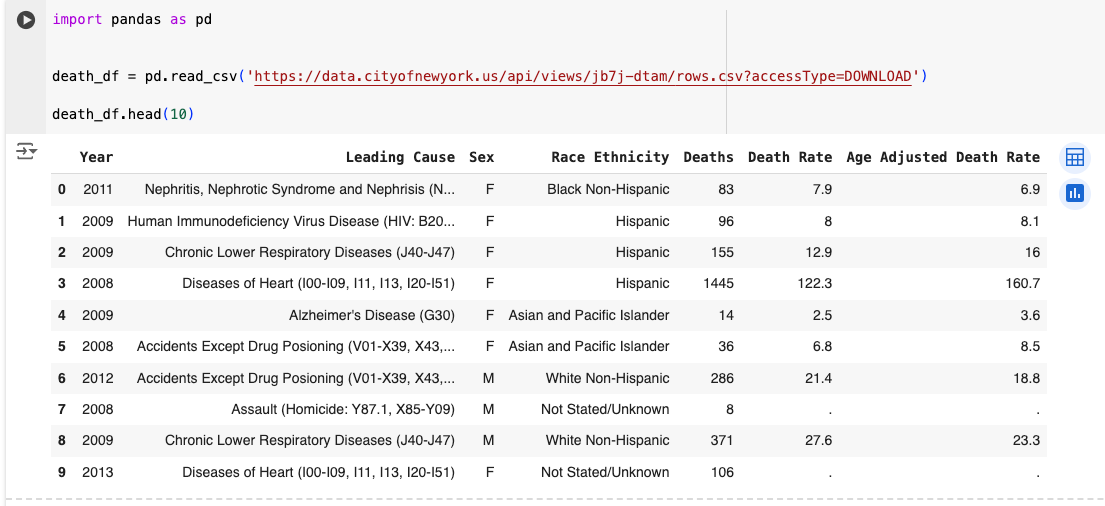
We create the name for the data frame and call it death_df.
Then we use pandas to read the CSV file we just uploaded and we paste the file path we just copied within the parenthesis (don’t forget to put quotation marks around the path).
Then we just print the first ten rows of our data frame using death_df.head(10).
Voila!
This is a real data frame made by the officials in the City of New York. It contains facts about deaths in NYC within a span of more than 10 years.
You can see immediately what kinds of features does it have. Besides the leading cause of death, it shows sex, ethnicity, number of deaths, death rate, and age adjusted death rate.
Perhaps we don’t need all the columns here. Let’s just use five of them. We can select parts of our data frame using this code:

Here I am overwriting the initial death_df data frame by selecting only 5 columns from it. I use the double square brackets to name the columns I want. I print the first 10 rows again to see it.
Now, let’s gain some insight into this data frame:

As it often happens, data frames will require some work before we’re able to do analysis. Sometimes they will contain a lot of missing values, have mistakes, misspellings, and other errors that might require cleaning and rearranging their inputs.
One thing that strikes us about this dataframe is that all columns are objects, except the ‘Year’, which is integer. While it makes sense that ‘Sex’ or ‘Race Ethnicity’ columns are objects, it doesn’t make sense for the number of deaths to be an object. In order to do any meaningful analysis, we’ll have to change the value of this column to some numeric value. Integers make the best sense, since they are whole values (we cannot have 1.5 people dead, for example).
Let’s change that before we proceed further:

Here, I overwrote the deaths column by assigning it as a new type (int for integer) of data. I also checked the info again to verify that the column is changed to integers.
Example of Data Analysis
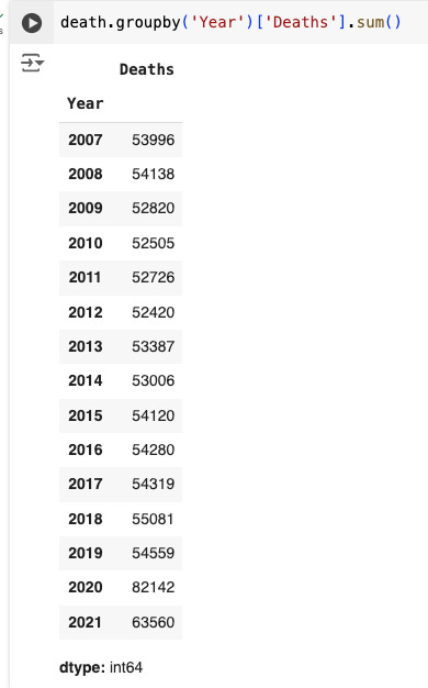
Now, one thing that we can do as an example of data analysis of this data frame, is to group deaths by year. If we do that, we may gain some insight that might be interesting or valuable.
We use the following code:
There you go. Your first act of data analysis is here!
Go through the code carefully to understand what is going on. First I type the name of the entire data frame, death, then I add a dot and type in .groupby(). This is called a method, and it works like a function of sorts. In this case it groups the data frame based on what column you specify in the parenthesis.
Here I used death.groupby(‘Year’) because I wanted to group something by years.
What do I want to group by year? That is specified in the next part of the code, which comes in the square brackets, where I specify what exactly I want to group by year, and that is the number of deaths. Finally, after specifying what I want grouped by year, I add another method .sum(), which simply adds all the deaths from each cause every year.
Finally, the whole piece of code looks like this:
death.groupby(‘Year’)[‘Deaths].sum()
You can see that functions are stacked on the data frame one by one (or appended to it with a dot before each function) to produce the desired outcome.
It reminds me of German language in the way meaning is generated by stacking short words to make a long one. Heres’s a funny one:
Donaudampfschifffahrtsgesellschaftskapitän
and it means ‘Danube steamship company captain’. Instead of four words to describe this role, Germans prefer to have a single word.
I love both German and Python.

Exercise 4: Study the deaths grouped by year. What interesting pattern do you notice? Anything sticking out? What?Let’s do a bit more. Now, let’s group the data by ‘Race Ethnicity’ column. We do it in the same way, but let’s make our analysis easier by ordering the output by size.
How do we do it?
We just stack another function at the end as Germans would, one that will sort the values, like this:

The sort_values() function orders the output ascending (lowest value first) by default, that’s why we have to specify that we want the values in descending (highest value first) order with sort_values(ascending = False).
Which group has the most deaths? What do you think why is that the case? What would be a good way to compare deaths across different ethnic groups?
Exercise 5: Group the data by 'Sex'. Notice a discrepancy? What is the discrepancy? Describe in one sentence/paragraph how would you clean and rearrange this data frame better before grouping it.

Exercise 6: Group the data by 'Leading Cause' with descending order. What was the leading cause of death?
Conclusion
We have barely scrached the surface of the functionality and usefulness of data frames for gaining insight, but I hope at least that you got something out of this lesson.
Nobody who wants to be a critical thinker in our times should skip learning about data, data frames, databases, and data analysis.
We live in a world where data analysis is an integral part of any complex task, be it scientific or commercial. Understanding what lies beneath is an imperative if you want to be a successful professional in any field.
If this is your first entry into this topic and you’d like to know more, you can continue your journey by reading some of the following books:


![Data Science from Scratch: First Principles with Python [Book]](https://substackcdn.com/image/fetch/f_auto,q_auto:good,fl_progressive:steep/https%3A%2F%2Fsubstack-post-media.s3.amazonaws.com%2Fpublic%2Fimages%2F50586a34-6e84-4734-ac09-8e03550ad774_1951x2560.jpeg "Data Science from Scratch: First Principles with Python [Book]")
Otherwise, I’ll see you in the next lesson.
Cheers!